---
title: "Tutorial at CMStatistics 2019"
author: "Jochen Einbeck"
output:
html_document:
df_print: paged
pdf_document: default
html_notebook:
df_print: paged
word_document: default
---
## Software requirements
It is strongly recommended that you use RStudio for this course, with R version $>=$ 3.2.3 installed.
For the use of R Notebooks we will need the packages`rmarkdown` and `knitr`. In principle, RStudio should automatically install these when required, but it may be a good idea to do this prior the start of the course, in RStudio, via `install.packages("rmarkdown", "knitr")`. Later in this course we will also require R packages `OpenImageR`, `arrayhelpers`, `LPCM`, `pracma`, and `GMCM`.
Other editors than RStudio (Tinn-R, emacs, etc) can be used if you prefer and *if you know how to use them*, but they will not supported in the course.
## Resources
The full material for this course includes
* this html document (this is "knitted" R notebook);
* a [raw](http://www.maths.dur.ac.uk/~dma0je/PG/Mix/TutorialCM19.Rmd) version of this notebook, `TutorialCM19.Rmd`, which you will use for your practical work;
* a [complete](http://www.maths.dur.ac.uk/~dma0je/PG/Mix/SolutionsCM19.Rmd) version of this notebook with solutions (to be updated sequentially after each coffee break);
* a [Handout](http://www.maths.dur.ac.uk/~dma0je/PG/Mix/HandoutCM19.pdf) (PDF) giving basics of R programming, and details on the methodolology for mixture modelling;
* the [Slides](http://www.maths.dur.ac.uk/~dma0je/PG/Mix/SlidesTutorialCM19.pdf) (PDF) for the lecture "The EM Algorithm for Finite Gaussian mixtures" (the lecture will be given before we begin with Part II of the morning session).
## Preparation
Please create somewhere on your computer an empty directory with title `CM19Tutorial`. This will be our *working directory*.
[Download](http://www.maths.dur.ac.uk/~dma0je/PG/Mix/TutorialCM19.Rmd) the file `TutorialCM19.Rmd` (use the right mouse button), and place it in the directory that you have just created. Then open it in RStudio, by double-clicking on that file. If you had already opened this file without having created the directory, please close it again, create the directory, place this file in there, and open the file as described.
We will use this .Rmd file to work through the tasks and examples in this tutorial.
------
# Part I (Tutorial 1)
## Objectives of Part I (before the 11:00 coffee break)
* using R Notebooks;
* workspace handling;
* reading in data;
* working with vectors, matrices, and data frames;
* basic programming devices (such as if...then, for, while, apply, functions);
* application to real data sets, including data from the energy sector.
## Using R Notebooks
This is a R Notebook. It is based on R Markdown and can be used for parallel typesetting and coding. It is best used in RStudio.
We are now continuing our work using the .Rmd file of the notebook, rather than the html version. You can of course still use the html file alongside.
There are (basically) three ways of executing (`rendering') code from a R Notebook.
* Chunk-by-chunk: A chunk of R code takes the shape (some random example code!)
```{r}
x<-3
x
D<- date()
D
DayofWeek<- substr(D, 1,x) # extracts the first x letters from date object
cat("Today's day of the week is:", DayofWeek)
```
which you can execute by clicking on the green triangle at the top right of the chunk. **DO THIS**.
* Row-wise. Click on any row of the code and then CTRL-ENTER. **DO THIS** for any of the rows in the chunk above.
* You can render (`knit') the entire document, it produces a nice and tidy summary of all text, code, and results.
**TRY THIS NOW**, that is click on the 'Knit' button at the top of this window. You can choose any of PDF, HTML, Word, or Preview, as output options.
*Notes*: My recommendation would be to set this option to `Knit to HTML`. This will produce a .html file in your workspace that you can open separately. `Preview` does not actually execute any chunks, it just shows pre-existing output. `Knit to PDF` will only work if you have already LaTex (under Windows, typically MikTex) installed; otherwise pdflatex will be unvailable. (But please don't worry about this for the sake of this course.)
You can, of course, edit this document yourself. The syntax is largely self-explaining, detailed explanations are available at https://rmarkdown.rstudio.com/authoring_basics.html. Specifically, you can create your own chunks by clicking on the `Insert` icon (towards the right of top menu bar of this window). **DO THIS** (then fill the chunk with some toy content, and execute).
Hence, there is no need to save or copy outputs of today's work into Latex, MS Word, etc. This document itself will be able to reproduce all your work done today.
The best way to carry out Part I of this course is to go chunk-by-chunk.
## Workspace handling
Every R session uses a *working directory*. This is some directory on your hard drive (or USB key, etc.) which R will use in order to save images, data, and your *workspace* (see below). R will also assume by default that any data sets that you attempt to read in are stored in this directory. By default, R Notebook chunks will use the location of the .Rmd file as working directory.
Check the content ("workspace") and location of the current working directory via
```{r}
ls()
getwd()
```
The first command should return you the output`x`, `D` and `DayofWeek`. (If that is not the case, then you can clean your global environment via `rm(list=ls())`.
The second command should return you the directory `ASMLTutorial` that you have created above. If this is not right, then the easiest way of fixing this is to close this .Rmd file and start again.
*Notes*:
* The working directory used within R chunks can be different from the working directory used by your current R console. For us, only the directory used by the chunks is of relevance.
* If you are already somewhat familiar with R then you will know that the R working directory can, in principle, be changed via `setwd("pathname")`. However, this will not work for R Notebooks, as it will only change the directory of the current chunk! More experienced users can follow these [instructions](https://philmikejones.me/tutorials/2015-05-20-set-root-directory-knitr/) to change the working directory for all R chunks.
You can, at any time, save the entire workspace for later use, by using the command `save.image("filename")`. Let's do this. Render
```{r}
save.image("cm19tut.RData")
```
then close RStudio and open it again. Then load the saved workspace back via
```{r}
load("cm19tut.RData")
ls()
```
and check whether everything is there! (In our case it should obviously just be `x`, `D` and `DayofWeek`.)
*Important (but rather confusing)*: RStudio opens a new R session to knit your R Notebook file. That is, even if you have some other objects (for instance from previous work) in the global environment (see top right RStudio window) then those objects will not be available when you knit your notebook. To see this, type for instance `test<-1` in your R console. You will see it shows up directly in the Global Environment. But, if you create a chunk which refers to `test` and then knit the notebook, you get an error.
## Reading in Data
The first data set that we are going to investigate give the energy use (kg of oil equivalent per capita) over 135 countries from 1960 to 2010.
*Energy use* is defined as the use of primary energy before transformation to other end-use fuels, which is equal to indigenous production plus imports and stock changes, minus exports and fuels supplied to ships and aircraft engaged in international transport.
Source: [Worldbank](http://data.worldbank.org/indicator/EG.USE.PCAP.KG.OE)
You can read the data in via
```{r}
energy.use <-read.csv("http://www.maths.dur.ac.uk/~dma0je/Data/energy.csv", header=TRUE)
```
Alternatively, you can download the data from the given web address, place them in your working directory, end then call `energy.use <-read.csv("energy.csv", header=TRUE)`.
Check now whether things have gone right. Try
```{r}
dim(energy.use)
```
which should give you the dimension $135 \times 12$. Also try
```{r}
head(energy.use)
```
in order to see the first six rows.
## Working with vectors, matrices and data frames
The object `energy.use` is a *data frame*. You can check whether or not an object is a data frame by typing `class(object)` or `is.data.frame(object)`. Try this for the object `energy.use` in the chunk below.
```{r}
class(energy.use)
is.data.frame(energy.use)
```
It is easy to access individual rows, columns, or elements of a data frame. For instance,
```{r}
energy.use[127,]
energy.use[,49]
energy.use[127,49]
```
will give you the 127th row; 49th column; and the entry of the 127th row and the 49th column, respectively (this is the UK energy consumption in 2007). You can also access columns directly through their column names, such as
```{r}
energy.use$X2007
```
Data frames are very important as they are the standard form in which data are expected by many R functions, such as
`lm`, `glm`,....
Let us now simplify the data frame a little bit, so that it is easier to use for the applied work. We reduce our interest to the energy consumption
in the years 2001 and 2007. We do this via
```{r}
energy <- energy.use[,c("X2001", "X2007")]
```
Also, we would like to give the rows and columns of the new data frame meaningful names. Please type
```{r}
rownames(energy)<- energy.use[, 1]
colnames(energy)<- c("use01", "use07")
```
in order to specify row and column names, respectively. Then type `energy` to look at your final data frame.
This data frame allows to access information quickly. For instance,
```{r}
energy["United Kingdom",]
```
gives you the UK values of energy consumption. **DO THIS** for a couple of countries.
```{r}
energy["Spain",]
```
## Basic programming devices
One may be interested in looking at these data in a form in which they are *ordered* by their energy consumption. This can be done using
```{r}
order(energy$use07)
```
which gives you a list of numbers. The first number tells you the index (here: 39) of the country with the smallest per-capita energy consumption (here: Eritrea), and typing `energy[order(energy$use07),]`
gives you the full ordered list.
In the chunk below, save this ordered data frame into a new data frame `senergy`.
```{r}
senergy <- energy[order(energy$use07),]
```
Next, we wish to identify the nations with extremely large energy consumption, say, more than 10000 kg of oil per capita (Intuitively, what do you think, which countries will this be?). Calling
```{r}
energy$use07 > 10000
```
will give you a vector of logical values, with a `TRUE` for each country for which this condition is met. The command
```{r}
sum(energy$use07 > 10000)
```
will tell you how many these are, and
```{r}
which(energy$use07 > 10000)
```
will give you the index numbers of these countries. From this, we would get the data rows corresponding to these countries via
```{r}
energy[which(energy$use07 > 10000),]
```
We would like to compare the energy use in 2001 and 2007. Do the same as above but now use the condition `energy$use01 > energy$use07` instead. Observe and understand the information that you gain at each step.
```{r}
energy$use01> energy$use07
sum(energy$use01> energy$use07)
which(energy$use01> energy$use07)
energy[which(energy$use01> energy$use07),]
```
A very useful tool to carry out repeated operations is the `for` command (see [Handout](http://www.maths.dur.ac.uk/~dma0je/PG/Mix/HandoutCM19.pdf)!).
Task: Implement a loop which, for all 135 countries, writes a text like
In 2007, the energy use in *country* was equivalent to *value* kg oil per capita.
```{r}
for (i in 1:135){
cat("In 2007, the energy use in ", rownames(energy)[i], " was equivalent to", energy[i,2], "kg oil per capita.", "\n")
}
```
Another command for repeated operations is `while`. It does not have a fixed number of loops, but proceeds until a certain condition is met. For instance, consider the ordered frame `senergy` created above. Assume we are interested in the following question: If we take exactly one person from each of the countries with the smallest energy use, i.e. one person from Eritrea, one person from Bangladesh, etc., then how many persons are needed in order to achieve the same use of energy as a single person in Qatar?
To answer this, create objects `i` and `sum07` and assign them the initial value 0. Then use the `while` function (see [Handout](http://www.maths.dur.ac.uk/~dma0je/PG/Mix/HandoutCM19.pdf)) with *condition* `sum07< senergy["Qatar",2]` and *action* `i <- i+1; sum07 <- sum07+ senergy[i,2]`. Make it clear to yourself what each row does. Also, interpret the result.
```{r}
energy["Qatar",]
i <-0
sum07 <-0
while(sum07< senergy["Qatar",2] ){
i=i+1
sum07<- sum07+ senergy[i,2]
}
i
sum07
# So individuals from the 41 least-consuming countries use less energy per captita than one single individual in Qatar!
```
Use `apply` to compute a vector which contains, for each country, the larger of the two energy consumption values given for 2001 and 2007. Consult the see [Handout](http://www.maths.dur.ac.uk/~dma0je/PG/Mix/HandoutCM19.pdf) and the corresponding help file (via `help(apply)`) if you are unsure how to do this.
```{r}
apply(energy,1,max)
```
Use `hist` and `boxplot` to create histograms and boxplots of the variables `use01` and `use07`. Comment on the distributional shape.
```{r}
boxplot(energy$use01, energy$use07)
par(mfrow=c(2,1))
hist(energy$use01)
hist(energy$use07)
```
Next, add logarithmic versions of these variables, say `luse01` and`luse07`, to the data frame via
```{r}
energy$luse01<- log(energy$use01)
```
and for`use07` analogously. Repeat the previous question using the transformed variables. What can we say about the distribution of these transformed variables, compared to the original ones?
```{r}
energy$luse07 <- log(energy$use07)
boxplot(energy$luse01, energy$luse07)
par(mfrow=c(2,1))
hist(energy$luse01)
hist(energy$luse07)
```
## Application and theory for finite Gaussian mixtures
Look again at your histogram from the `luse01` variable.
```{r}
par(mfrow=c(1,1))
hist(energy$luse01)
```
One may be interested in *modelling* this distribution, i.e. describing it through some parametric family of distributions. A Gaussian distribution appears to be inadequate due to the clear dip in the center. But, perhaps one could argue that *two* Gaussian distributions are involved here: One Gaussian centered at about 6.5, and another one centered at about 8.5, and both of them roughly equally likely. This leads to the idea of mixture modelling, to which we turn in this section.
Next, we consider a data set featuring $n=82$ observations of galaxy velocities. Load the `galaxies` data, read the associated help file, and create a histogram using the option `breaks =18` in function `hist`.
```{r}
data(galaxies, package="MASS")
?galaxies
hist(galaxies, breaks=18)
```
The histogram clearly tells that there are several modes (perhaps, 4 or 5) present in the data, each of them associated with strongly differing proportions of the total sample size. These different modes may be evidence for the presence of some unobserved heterogeneity, for instance due to the size or distance of the galaxies.
Here again, one could think of the distribution of the data as an overlay of several Gaussian density functions, but now with unequal probabilities. The general term for such a situation is a *Finite Gaussian mixture*. See the [Handout](http://www.maths.dur.ac.uk/~dma0je/PG/Mix/HandoutCM19.pdf) for details.
If you have arrived at this point before the lecture, then please take a paper and pencil, and attempt to derive equations (3), (4), and (5) on the [Handout](http://www.maths.dur.ac.uk/~dma0je/PG/Mix/HandoutCM19.pdf). You can do this by taking the appropriate derivatives of equation (8). Begin with the $\mu_k$.
Notes:
* Please attend the [Lecture](http://www.maths.dur.ac.uk/~dma0je/PG/Mix/SlidesTutorialCM19.pdf) **EM algorithm for finite Gaussian mixtures** before you proceed further.
* If you leave the computer now, don't forget to **save your workspace** as explained above.
------
# Part II (Tutorial 1)
## Objectives of Part II (before lunch)
* Introduction to Gaussian mixtures
* Apply programming skills from Part I
* Implement EM algorithm for Finite Gaussian mixtures
* Simulate from Finite Gaussian Mixtures
* Bootstrap: Testing for the number of components (optional)
## Implementing the EM algorithm for Gaussian mixtures
Implement now the EM-algorithm for finite Gaussian mixtures. You will need for this
* a function which implements the E-step. The framework for this function is
```{r}
estep<- function(dat, p, mu, sigma){
n <- length(dat)
K <- length(mu)
W <- matrix(0, n,K)
for (i in 1:n){
W[i,]<- p/sigma*exp(-1/(2*sigma^2)*(dat[i]-mu)^2)/ sum( p/sigma*exp(-1/(2*sigma^2)*(dat[i]-mu)^2))
}
return(W)
}
```
This function takes the data $y={\tt dat}$ and the current parameter estimates $\hat{\theta}=({\tt p, mu, sigma})$ as arguments, and produces the matrix ${\tt W}=(w_{ik})_{1\le i \le n, 1\le k \le K}$. Note that `p`, `mu` and `sigma` are vectors.
* another function which implements the M- Step:
```{r}
mstep<- function(dat, W){
n <- dim(W)[1]
K <- dim(W)[2]
p <- apply(W,2,sum)/n
mu<- apply(W*dat,2,sum)/apply(W,2,sum)
diff<-matrix(0,n, K)
for (k in 1:K){
diff[,k]<- (dat -mu[k])^2
}
var <- apply(W*diff,2,sum)/apply(W,2,sum)
sigma <- sqrt(var)
return(list("p"=p, "mu"=mu, "sigma"=sigma))
}
```
*Note*: There are several ways to implement the estimate of $\sigma_k$, but without advanced programming expertise you will probably need some iterative way of doing this. For instance, one can loop over $i$ and add the relevant contribution at each stage. Or, one can firstly construct a $n\times K$ matrix, say `diff`, of squared differences $(y_i-\mu_k)^2$, and then use `apply(W*diff, 2, sum)`.
* a third function which makes the actual EM-algorithm; something like
```{r}
em <- function(dat,K, steps=400){
#pb<-txtProgressBar(min=0, max=steps, style=3)
p <- rep(1/K,K)
mu <- quantile(dat, probs= (1:K)/K-1/(2*K))
sigma <- rep(sd(dat), K)
s<-1
while (s <=steps){
W <- estep(dat, p, mu, sigma)
fit <- mstep(dat, W)
p <- fit$p
mu <- fit$mu
sigma <-fit$sigma
s<-s+1
#setTxtProgressBar(pb,s)
}
fit<- list("p"=p, "mu"=mu, "sigma"=sigma, "W" =W)
return(fit)
}
```
Apply your implemented algorithm on the `luse01` and `galaxies` data.
```{r}
test1 <- em(galaxies, K=4)
test2 <- em(energy$luse01, K=2)
```
Once your function works, we propose an helpful improvement: It is often useful to track the number of iterations, so that you know which proportion of the total runtime has already been completed. You can do this through a *progress bar*. Include directly at the start of the body of `em` the line `pb<-txtProgressBar(min=0, max=steps, style=3)`, and then before the while loop `setTxtProgressBar(pb,s)`. After adding these, re-run the two examples and observe the result.
## Visualization
In order to visualize the fitted mixture, you can use the following function (for the purposes of this course, you don't need to worry about the content of this function; just take it as it is. The names of the function arguments are self-explanatory.)
```{r}
plot.mixND<- function(dat, p, mu, sigma, breaks=25, dens=TRUE, ngrid=401, ...){
try<- hist(dat, breaks=breaks, plot=FALSE)
hist(dat, breaks=breaks, freq=FALSE, ylim=c(0, max(try$density)*1.3),
col="grey93" , border="grey85",...)
r <- diff(range(dat))
grid<- seq(min(dat)-0.15*r, max(dat)+0.15*r, length=ngrid)
K<- length(p)
if (length(sigma)==1){
sigma<-rep(sigma, K)
}
grid.mat<- matrix(0, ngrid,K)
for (j in 1:K){
grid.mat[,j]<- p[j]*dnorm(grid, mu[j], sigma[j])
}
for (j in 1:K){
lines(grid, grid.mat[,j], col=j+1, lwd=2)
}
if (dens){
lines(grid, apply(grid.mat,1, sum), col=1,lwd=2)
}
invisible()
}
```
Apply this function onto the two fitted models. Play around with the provided graphical options to understand their effect.
```{r}
plot.mixND(galaxies, test1$p, test1$mu, test1$sigma, main="galaxies", xlab="galaxies", dens=FALSE)
plot.mixND(energy$luse01, test2$p, test2$mu, test2$sigma, main="energy use", xlab="log(energy use)", dens=FALSE)
```
*Note*: If you have arrived at this point, then the core objective of the morning part of the course is achieved: You have your own EM algorithm running and have displayed the output! The parts which follow are useful add-ons, which are partially a bit more advanced and challenging.
## Simulation and Bootstrap
Read the section on Simulation given on the [Handout](http://www.maths.dur.ac.uk/~dma0je/PG/Mix/HandoutCM19.pdf), then complete the missing code line below to implement a simulator which generates a *single* observation from a Gaussian mixture:
```{r}
gauss.mix.sim1 <- function(K, p, mu, sigma){
x <-runif(1)
sim <- 0
cpi <- cumsum(pi)
k <-1
while (x>cpi[k]){
k<-k+1
}
sim <- rnorm(1,mu[k],sigma)
return(sim)
}
gauss.mix.sim1(2, c(0.5,0.5), c(1/4,3/4),1/2) # Example for application
```
Extend the code and write a function `gauss.mix.sim` which simulates an arbitrary number, say `n`, of replicates. Try your function using a value of $\theta$ of your choice, plot the histogram,
and observe whether the result looks right.
```{r}
gauss.mix.sim<-function(n, K, pi, mu, sigma){
x<-runif(n)
sim<-rep(0,n)
cpi<-cumsum(pi)
for (i in 1:n){
k <-1
while (x[i]>cpi[k]){
k<-k+1
}
sim[i] <- rnorm(1,mu[k],sigma)
}
return(sim)
}
save<-gauss.mix.sim(100,2, c(0.5,0.5), c(-1,1),1/2) # Example for application
hist(save)
```
Improve your function `em` so that it returns the likelihood and the disparity as additional outputs.
Read the instructions in the [Handout](http://www.maths.dur.ac.uk/~dma0je/PG/Mix/HandoutCM19.pdf) before your attempt this. Call the new function `EM`.
```{r}
EM <- function(dat,K, steps=400, tol=1, showbar=TRUE){
if (showbar) {pb <- txtProgressBar(min=0, max=steps, style=3)}
p <- rep(1/K,K)
mu <- mean(dat)+tol*quantile(dat-mean(dat), probs= (1:K)/K-1/(2*K))
sigma <- rep(sd(dat), K)
s<-1
while (s <=steps){
W <- estep(dat, p, mu, sigma)
fit <- mstep(dat, W)
mu <- fit$mu
p <- fit$p
sigma<- fit$sigma
s<-s+1
if(showbar) {setTxtProgressBar(pb,s)}
}
dens.all<-matrix(0,length(dat), K)
for (k in 1:K){
dens.all[,k]<- p[k]*dnorm(dat, mu[k],sigma[k])
}
loglik<- sum(log(apply(dens.all,1,sum)))
fit<- list("p"=p, "mu"=mu, "sigma"=sigma, "wik" =W,"data"=dat, "disp"=-2*loglik )
class(fit)<-"EM"
return(fit)
}
```
Now apply the function onto `galaxies` and `energy$luse01`.
```{r results="hide"}
fit1 <- EM(galaxies, K=4, showbar=TRUE)
fit2 <- EM(energy$luse01, K=2, showbar=TRUE)
```
```{r}
fit1[c("p", "mu", "sigma", "disp")]
fit2[c("p", "mu", "sigma", "disp")]
```
Then, implement the likelihood ratio test for testing for the number of mixture components $K$, following the instructions provided on the [Handout](http://www.maths.dur.ac.uk/~dma0je/PG/Mix/HandoutCM19.pdf) (Consider the inclusion of a progress bar for the number of bootstrap iterations).
```{r results="hide"}
# H_0: K components
# H_1: K+1 components
n <- length(galaxies)
fit4 <- EM(galaxies, K=4)
fit5 <- EM(galaxies, K=5)
LRTS <- fit4$disp-fit5$disp
M <- 99
sim.LRTS <-rep(0,M)
pbB<-txtProgressBar(min=0, max=M, style=3)
for (m in 1:M){
sim4 <- gauss.mix.sim(n, 4, p=fit4$p, mu=fit4$mu, sigma=fit4$sigma)
fit.sim4<- EM(sim4,4, steps=100, showbar=FALSE)
fit.sim5<- EM(sim4,5, steps=100, showbar=FALSE)
sim.LRTS[m]<- fit.sim4$disp-fit.sim5$disp
setTxtProgressBar(pbB,m)
}
```
From this, the remaining step is to find the bootstrapped p-value:
```{r}
pval <- 1-rank(c(LRTS, sim.LRTS))[1]/100
pval
```
# Part III (Tutorial 2)
## Objectives of Part III (after lunch)
* Introdution to clustering techniques
- Gaussian mixtures (EM)
- k-means
- Mean shift
* Basics of image analysis
- Types of images
- How to read in images
- How to prepare image data for analysis/manipulation
- How to transform data back to an image
* Use clustering techniques for image segmentation
- Clustering in grey scale phase space
- Reconstruction of segmented image
- Mode filtering
- Clustering in 3D RGB space
- Further optional and advanced topics...
**Feel free to complete Parts I and II in the afternoon session if not finished so far.**
The first task in any image analysis is, clearly, to read the image in.
We will need two R packages to help us a bit: One to "open" the images, and one to rearrange the data imported from them. Please load the two following packages. [You will need, firstly, to install the packages via `install.packages("..")` if not done so already.]
```{r}
require(OpenImageR)
require(arrayhelpers)
```
Now we download, open, and visualize the image.
```{r}
download.file("http://www.maths.dur.ac.uk/~dma0je/PG/Mix/cliffs.jpg", destfile="cliffs.jpg", mode="wb")
cliffs0 <- readImage("cliffs.jpg")
imageShow(cliffs0)
```
Note: On some systems I have seen that `imageShow` and R Markdown don't work well together, so that nothing happens here. In this case please just run `imageShow(cliffs)` again in the Console (for instance, by hitting the Shift button) and you should see the image.
It is useful to understand a few things about image files here. On a basic level we distinguish grey scale and color images.
**Grey scale images** will usually either come
* as a matrix (such as 1024 x 1024) of grey scale values between 0 and 1, where 1=white and 0=black
* or as a pseudo-color image which consists of three identical copies of the grey scale image; for instance we see that for the `Cliffs` image we have
```{r}
dim(cliffs0)
```
Now, note that all three layers contain the same content; e.g.
```{r}
sum(cliffs0[,,1]==cliffs0[,,2])
```
We can in this case use any of the three copies to obtain the grey scale image, such as done above through
```{r}
cliffs1 <- cliffs0[,,1]
imageShow(cliffs1)
```
It should be said that `imageShow` has taken out some of the difficulty here. There is a deeper-laying twist: A matrix value [i,j] is defined by running the index `i` *downwards vertically*, then `j` *rightwards horizontally*. However, an image coordinate is defined by a horizontal coordinate, then a vertical (upwards) coordinate. The function `imageShow` has carried out this transformation in the background. If we hadn't this available, we would need to do this manually:
```{r}
# rotate <- function(x){t(apply(x, 2, rev))}
# image(rotate(cliffs1), col=gray.colors(500))
```
(This takes a while!)
For **color images**, the three layers of the array will usually refer to the RGB values. Let us read in another image:
```{r}
require(OpenImageR)
download.file("http://www.maths.dur.ac.uk/~dma0je/PG/Mix/france.jpg", destfile="france.jpg", mode="wb")
france0 <- readImage("france.jpg")
imageShow(france0)
```
Now we have
```{r}
dim(france0)
sum(france0[,,1]==france0[,,2])
```
If you need to convert a color image to a grey scale image, the three layers can be weighted via 0.21 R + 0.72 G + 0.07 B (Luminosity method). Let's do this.
```{r}
france1<- 0.21*france0[,,1]+0.72*france0[,,2]+0.07*france0[,,3]
imageShow(france1)
```
We return, for now, to the analysis of grey scale images, and continue with preparing the image with the cliffs for statistical processing. Firstly, the current 1024 x 1024 image is still quite large to deal with. We resize it via
```{r}
cliffs <- resizeImage(cliffs1, 256, 256, method = "nearest")
dim(cliffs)
imageShow(cliffs)
```
We then need to transform the matrix into an array
```{r}
Cliffs<- array2df(cliffs)
dim(Cliffs)
names(Cliffs)
head(Cliffs)
```
where the first column contains the grey scales and the other two columns contain the coordinates. We can visualize the grey scale distribution through a histogram:
```{r}
hist(Cliffs$cliffs)
```
We see that there are three or four clusters in the data, with the leftmost bar representing the black image frame.
To identify the clusters, any clustering method can be used. We begin with k-means. See for instance [this resource](https://bigdata-madesimple.com/possibly-the-simplest-way-to-explain-k-means-algorithm/) for a quick introduction into this algorithm.
```{r}
fitcliffs.KM<- kmeans(Cliffs$cliffs, 4)
names(fitcliffs.KM)
```
The relevant results (for us) are in the component `$centers`, which gives the three cluster centers, and the component `$cluster`, which tells which center is closest to each data point.
```{r}
fitcliffs.KM$centers
table(fitcliffs.KM$cluster)
```
The trick of cluster-based image segmentation is now, for each pixel, to *replace the original grey scales by the grey scale corresponding to their respective cluster center*. This can be done very efficiently given the k-means output:
```{r}
post.cliffs.KM<- fitcliffs.KM$centers[fitcliffs.KM$cluster]
table(post.cliffs.KM)
```
Finally, the long vector of grey scales needs to be transformed back into an image. Being unaware of an existing, automated function for that purpose, I provide one:
```{r}
vector2image <- function(image.vector, show=TRUE, width=NULL){
N<-length(image.vector)
D<- sqrt(N)
if (is.null(width)){
if ((D %%1) !=0){
stop("This is not a square image so you need to give the image width")
} else {
width<- D
}
}
height<- N/width
image.matrix<- matrix(image.vector, nrow=height, ncol=width)
if (show) {
require(OpenImageR)
imageShow(image.matrix)
}
return(image.matrix)
}
```
Then, we reconstruct the `segmented' image via
```{r}
KM.cliff.image<- vector2image(post.cliffs.KM, show=FALSE)
dim(KM.cliff.image)
imageShow(KM.cliff.image)
```
(The same problem that we had with `ImageShow` before also manifests itself here -- you may need to re-execute the call on the command line in order to see the image.)
We see that the segmentation is not very good. A first attempt could be to change the type of algorithm used to execute k-means.
This can be done through the option `algorithm` in function `kmeans`, for instance to `"Lloyd"` or ` "MacQueeen"`. **Try this**!
```{r}
# ?kmeans
# ...
```
Larger differences in segmentation can be expected when going for an entirely different clustering algorithm. Let us now use EM for Gaussian mixtures as implemented previously.
```{r}
fitcliffs.EM<- EM(Cliffs$cliffs, K=3, steps=200)
fitcliffs.EM[c("p", "mu", "sigma")]
```
```{r}
plot.mixND(Cliffs$cliffs, fitcliffs.EM$p, fitcliffs.EM$mu, fitcliffs.EM$sigma, dens=FALSE)
```
We clearly see the fitted three components. The next task, is, again, to replace the original grey scales by the grey scale corresponding to their respective cluster center. For mixtures, this is done by allocating *each observation that component to which it belongs with highest probability*. This information is contained in the weight matrix `W`, that is
```{r}
head(fitcliffs.EM$wik)
```
It is cumbersome to carry out this processing step manually, so we devise a function for it.
```{r}
post.em<-function(mu, W){
n<- dim(W)[1]
K<- dim(W)[2]
post.image.class<- rep(0,n)
post.image.tone <- rep(0,n)
for (i in 1:n){
post.image.class[i]<-which.max(W[i,])
}
post.image.tone <- mu[post.image.class]
return(list("class"=post.image.class, "tone"=post.image.tone))
}
```
Now, we can execute
```{r}
post.cliffs.EM<- post.em(fitcliffs.EM$mu, fitcliffs.EM$wik)$tone
table(post.cliffs.EM)
```
Note this is a vector of length 65536 which only contains three different values. Finally, the vector needs to be mapped back to a matrix. We do this again through our function `vector2image`:
```{r}
EM.cliff.image<- vector2image(post.cliffs.EM, show=FALSE)
dim(EM.cliff.image)
imageShow(EM.cliff.image)
```
You should now see the "segmented" image. You see, again, that the segmentation has only been a partial success, with a considerable proportion of "contaminating" pixels throughout the image. We will later learn how we can address this problem through an appropriate *filter*.
But before we do this, we will look at a third clustering method: Mean shift clustering. This clustering technique works by computing, for each observation, a sequence of local averages which eventally converges to a local mode of the data density. See for instance [this resource](https://spin.atomicobject.com/2015/05/26/mean-shift-clustering/) for an intuitive introduction into this technique.
To illustrate this, let's simply do this for the Old Faithful Geyser data
```{r}
require(LPCM)
ms(faithful)
```
Unfortunately, mean shift clustering is quite slow, so I have to provide an accelerated version; `the mop-up meanshift':
```{r}
source("http://www.maths.dur.ac.uk/~dma0je/PG/Mix/ms.mopup.r")
```
The idea of this variant of the mean shift algorithm is to classify all observations which are "close" to an existing mean shift trajectory (within one bandwidth) to the mode to which that trajectory had converged.
Now, we can run the following code sequence, similar as above for the k-means
```{r, echo=TRUE}
fitcliffs.MS<- ms.mop(Cliffs$cliffs, scaled=0, h=0.045)
names(fitcliffs.MS)
fitcliffs.MS$cluster.center
post.cliffs.MS<- fitcliffs.MS$cluster.center[fitcliffs.MS$cluster.label]
MS.cliff.image<- vector2image(post.cliffs.MS, show=FALSE )
dim(MS.cliff.image)
imageShow(MS.cliff.image)
```
which gives a relatively good segmentation. Note that the numbers which are displayed, when using `ms.mop`, are the number of remaining points which are left to cluster after each iteration.
## Mode filtering
The idea of a mode filter is to get rid of little contaminations within segments by replacing such "contaminated" pixels with a majority vote of neighboring pixels. A simple implementation of a mode filter is given below.
```{r}
neighbors<-function(d1,d2, j,k, include.center=TRUE){
neigh<-matrix(NA,0,2)
if (include.center){
neigh<-rbind(neigh, c(j,k))
}
if (j>1){neigh<-rbind(neigh, c(j-1,k))}
if (j1){neigh<-rbind(neigh, c(j, k-1))}
if (k100000 pixels! An R function which can still deal which such situations reasonably quickly is `EMAlgorithm` in R package `GMCM`. For some literature on RGB clustering via Gaussian Mixtures, see https://www.researchgate.net/publication/250791017_Image_Segmentation_using_Gaussian_Mixture_Models
* Similarly, also the mean shift struggles in RGB space to deliver a result in a reasonable time; even in the mop-up version. If you use function `mop.up`, use bandwidths of at least `h=0.05` and option `mult.opt=2` (this implies that all observations which are less than two bandwidths away from any mean shift trajectory will automatically get classified to the mode to which that trajectory had converged.)
Place your attempts in the chunk below.
(Example for mop-up mean shift application on France data provided).
```{r}
# fitfrance.MS<- ms.mop(France, scaled=0, h=0.05, mop.mult=3)
# names(fitfrance.MS)
# fitfrance.MS$cluster.center
# post.france.MS<- fitfrance.MS$cluster.center[fitfrance.MS$cluster.label,]
# head(post.france.MS)
# MS.france.image<-array(0,dim=dim(france0))
# dim(MS.france.image)
# for (j in 1:3){
# MS.france.image[,,j]<- vector2image(post.france.MS[,j], width=445)
# }
# imageShow(MS.france.image)
```
## Evening session and prize
The time after the last coffee break is entirely dedicated to your own hands-on work. Please use either one of the provided images, or any other images that you find on your computer / phone / the internet (noting copyright restrictions!), and apply the techniques discussed in here.
If you struggle to find good images, you may use the [Berkeley Segmentation Dataset](https://www2.eecs.berkeley.edu/Research/Projects/CS/vision/grouping/segbench/BSDS300/html/dataset/images.html).
**For the best segmentation of ANY image, I will give out at the end a (brandnew) T-Shirt relating to a recent postgraduate training event at Durham University**
The prize was won by Christian Capezza, for this image
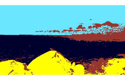.
Despite still showing some impurities, this segmentation clearly identifies the main three features of the image: sky, sea and rocks, plus an additional segment for "everything else" which was not classifiable into any of these three segments. The associated code is given below (note the code is not deterministic!).
```{r}
# France3 <- France
## use logit scale, but deal with 0 and 1 whose logit is infinite.
# France3[France3 == 0] <- jitter(0)
# France3[France3 == 1] <- jitter(1, amount = .05)
# France3 <- cbind(logit((France3 / diff(range(France3)) - min(France3)) * .99 + .005), France0$d1[1:111250], France0$d2[1:111250])
## this is adding the pixel coordinates as additional features
# library(GMCM)
# out <- EMAlgorithm(France3, m = 4)
# out$cluster <- apply(out$kappa, 1, which.max)
# out$centers <- do.call(rbind, out$theta$mu)
# post.france.GMCM <- out$centers[out$cluster,]
# GMCM.france.image<-array(0,dim=dim(france0))
# for (j in 1:3){
# GMCM.france.image[,,j]<- vector2image(post.france.GMCM[,j], width=445)
# }
# imageShow(GMCM.france.image)```
```
## Improve your results (1)
In order to improve any of your segmentations achieved so far, please consider the following options:
* changing the clustering method;
* changing the number of clusters of any of the methods (or, in case of the mean shift, change the bandwidth);
* investigating the effect of other settings, such as EM starting points, or k-means variants.
You will probably achieve a modest, but not massive, improvement through these attempts. For more substantial improvements, you need to engage with the techniques further below.
```{r}
# ...
```
## Improve your results (2)
* Increase and improve the range of features (variables) used for the clustering, such as
- spatial coordinates; e.g. (https://courses.csail.mit.edu/6.869/handouts/PAMIMeanshift.pdf);
- variables representing the `texture' of the image, see e.g http://www.maths.dur.ac.uk/~dma0je/Lit/Coleman-Andrews.pdf;
- use transformations of the RGB color space into Luv or HSV, see e.g. https://www.researchgate.net/publication/251465117_Color_Spaces_and_Image_Segmentation;
* Improve the filtering, e.g. by
- considering modes over larger patches; e.g. http://www.maths.dur.ac.uk/~dma0je/Lit/mode-filter.pdf;
- invert the order of the segmentation and the mode filtering;
- use a *mean filter* or *median filter* instead of the mode filter (Note that these only really make sense *before* rather than *after* the segmentation)
* Look out for off-the-shelf machine learning tools on R or elsewhere...
```{r}
# ...
```
## What's the use of my segmentation?
See https://uk.mathworks.com/discovery/image-segmentation.html for some nice and light reading!
## Thanks for your participation!
Any questions, contact jochen.einbeck@durham.ac.uk