These notes assume familiarity with vector calculus, in particular
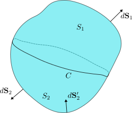
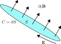
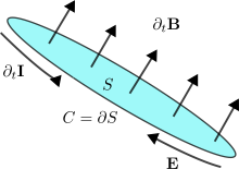
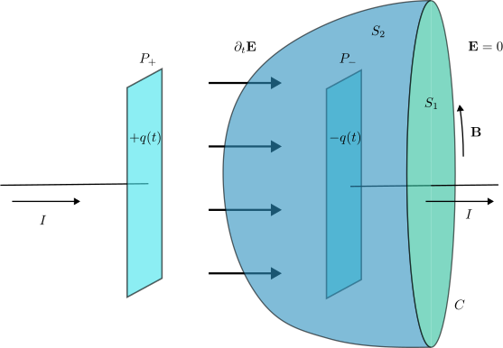
Gauss’ theorem and Stokes’ theorem, as covered in Mathematical Methods
II (MATH2811). Two appendices collect background material on vector
calculus and on Dirac’s delta function. A third appendix contains
derivations used in Section 2.2.
Latin indices (\(a,b,i,j,\dots\)) run from \(1\) to \(3\).
Greek indices (\(\alpha,\beta,\mu,\nu,\dots\)) run from
\(0\) to \(3\).
For partial derivatives we write \(\partial_\mu \equiv \frac{\partial}{\partial
x^\mu}\) and \(\partial_\mu^\prime
\equiv \frac{\partial}{\partial x^{\mu^\prime}}\).
Unless stated otherwise, all fields are smooth and we freely
commute partial derivatives.
For the three-dimensional Levi–Civita symbol we take \(\varepsilon_{123}=1\).
These notes are intended to be self-contained. For additional
reading, the following textbooks are excellent references,
D. J. Griffiths, Introduction to
Electrodynamics.
E. M. Purcell and D. J. Morin, Electricity and
Magnetism.
J. D. Jackson, Classical Electrodynamics.
1
Introduction
These lectures broadly follow the historical development of
electromagnetism, a theory for the electric and magnetic fields, sourced
by charge density \(\rho\) and current
density \(\mathbf{J}\). We begin with
time-independent configurations, where the subject naturally splits into
electrostatics and magnetostatics and where \(\mathbf{E}\) and \(\mathbf{B}\) can be treated as distinct
fields governed by separate laws.
We then turn to electrodynamics, where this separation breaks down.
Time dependence ties electric and magnetic phenomena together through
induction, and Maxwell’s completion of the classical laws shows that
\(\mathbf{E}\) and \(\mathbf{B}\) are intrinsically coupled
components of a single theory. In this sense, Maxwell’s theory,
was the first great example of unification in physics. It also brings
into view a new organising principle, gauge symmetry. We will
repeatedly see that gauge freedom is not merely a calculational
convenience, but a structural feature of the theory. After identifying
suitable degrees of freedom, we will connect with the first part of the
module and derive these equations from an action principle.
Finally, we refine this understanding by recognising that
electromagnetism fits naturally within special relativity. The
relativistic viewpoint clarifies how electric and magnetic fields
transform between inertial frames and makes the unity of the theory
manifest. It also motivates an efficient formulation in terms of
spacetime tensors, most notably the electromagnetic field tensor \(F_{\mu\nu}\), which packages \(\mathbf{E}\) and \(\mathbf{B}\) into a single
Lorentz-covariant object and leads naturally to a compact statement of
Maxwell’s equations.
2
Electric Charge and its Transport Properties
2.1
Charge and Current Density
Electric charge is a real number assigned to particles,
characterising how they interact with the electromagnetic field. Unlike
mass, charge can be positive or negative; a neutral particle does not
couple to electromagnetic fields. The SI unit is the Coulomb (C), which
is a large unit. Note that the electron has charge \(q=-e\) with \(e=1.6\cdot 10^{-19}\,\mathrm{C}\), while
quarks carry charges \(q=2e/3\) or
\(q=-e/3\).
In a point-particle description, charge is concentrated at isolated
points. In many applications, however, it is convenient to treat charge
as “smeared” along a wire, spread over a surface, or distributed
smoothly in space. To describe a time-dependent distribution of charge
we introduce the charge density\(\rho(t,\mathbf{x})\), which appears as a
source in Maxwell’s equations. By definition, \(\rho\) is charge per unit volume, so the
total charge contained in a region \(V\subset\mathbb{R}^3\) at time \(t\) is, \[\begin{align}
\label{eq:charge_def}
Q_V(t)=\int_V \rho(t,\mathbf{x})\,d^3\mathbf{x}\,.
\end{align}\]
Consider a point particle of charge \(q\) located at \(\mathbf{y}(t)\). The corresponding charge
density \(\rho(t,\mathbf{x})\) must
satisfy, \[\int_V
\rho(t,\mathbf{x})\,d^3\mathbf{x}=\begin{cases}
q& \mathrm{if}\,\, \mathbf{y}(t)\in V\\
0& \mathrm{if}\,\, \mathbf{y}(t)\notin V
\end{cases}\,.\] Using the defining property of Dirac’s delta
(Appendix 10), we can write \(\rho(t,\mathbf{x})=q\,\delta(\mathbf{x}-\mathbf{y}(t))\).
For \(N\) particles at positions \(\mathbf{y}_i(t)\) with charges \(q_i\), this generalises to, \[\begin{equation} \label{eq:point_particles_ch}
\rho(t,\mathbf{x})=\sum_{i=1}^N
q_i\,\delta(\mathbf{x}-\mathbf{y}_i(t))\,. \end{equation}\]
Electric current is the transport of charge. The current
density\(\mathbf{J}(t,\mathbf{x})\) is defined so
that, for an oriented surface \(S\),
the rate at which charge crosses \(S\)
is, \[\begin{align}
\label{eq:current_def}
I_S(t)=\int_S \mathbf{J}(t,\mathbf{x})\cdot d\mathbf{S}\,.
\end{align}\] As with \(\rho\),
one can describe currents confined to curves or surfaces, as well as
currents flowing throughout three-dimensional space; we discuss these
cases in more detail in the next subsection.
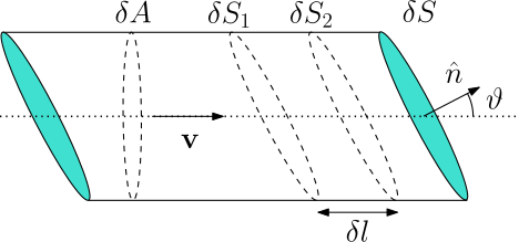
Flow of charged fluid through a small oriented surface
element \(\delta\mathbf{S}\).
A charged fluid is described by its charge density \(\rho(t,\mathbf{x})\) and by a velocity
field \(\mathbf{v}(t,\mathbf{x})\). The
associated current density is \(\mathbf{J}(t,\mathbf{x})=\rho(t,\mathbf{x})\,\mathbf{v}(t,\mathbf{x})\).
To see this, consider the geometry in Figure 1. Let \(\delta\mathbf{S}=\hat{\mathbf{n}}\,\delta
S\) be a small surface element with unit normal \(\hat{\mathbf{n}}\), and let \(\vartheta\) be the angle between \(\mathbf{v}\) and \(\hat{\mathbf{n}}\). In a short time \(\delta t\), the fluid travels a distance
\(\delta l=|\mathbf{v}|\,\delta t\)
along the direction of \(\mathbf{v}\).
The amount of fluid between surfaces \(\delta
S_1\) and \(\delta S_2\)
occupies a thin slab of volume, \[\delta
V=(\delta S\cos\vartheta)\,\delta l\,,\] and crosses \(\delta\mathbf{S}\). Note that we used that
\(\delta A= \delta S\cos\vartheta\) is
the area of the projection of the surface element perpendicular to the
flow. The charge carried by this volume is \(\delta Q=\rho\,\delta V\), hence, \[\begin{aligned}
\frac{\delta Q}{\delta t}=\rho\,\mathbf{v}\cdot \delta\mathbf{S}\,.
\end{aligned}\] Comparing with the definition \(\eqref{eq:current_def}\) gives \(\mathbf{J}=\rho\,\mathbf{v}\).
The electromagnetic field exerts a force density \(\mathbf{f}_{\mathrm{L}}=\rho\,\mathbf{E}+\mathbf{J}\times\mathbf{B}\)
on a charge density \(\rho\) and
current density \(\mathbf{J}\).
To show this result, consider a small fluid element of volume \(\delta V\). The total charge inside the
element can be approximated by \(\delta a=
\rho\,\delta V\) resulting in a Lorentz force \[\delta \mathbf{F}_{\mathrm{L}}=\delta
q\left(\mathbf{E}+\mathbf{v}\times \mathbf{B}\right)\,,\] where
\(\mathbf{v}\) is the fluid velocity of
the distribution. Substituting the expression for \(\delta q\) we have, \[\begin{aligned}
\delta
\mathbf{F}_{\mathrm{L}}&=\rho\left(\mathbf{E}+\mathbf{v}\times
\mathbf{B}\right)\delta V\\
&=\left(\rho\,\mathbf{E}+\mathbf{J}\times
\mathbf{B}\right)\delta V\,,
\end{aligned}\] where in the second line we used \(\mathbf{J}=\rho\,\mathbf{v}\), as we showed
in Example [ex:fluid_flow_cur_den]. The
last line proves the desired result.
A fundamental property is that electric charge can neither be
destroyed nor created, it can only move from one region to another1. This statement of local charge
conservation can be phrased as follows. Let \(V\) be an arbitrary volume with closed
boundary \(S=\partial V\). The rate of
change of charge in \(V\) is equal to
minus the net current flowing out through \(S\), \[\begin{align}
\label{eq:charge_cons}
\frac{d}{dt}Q_V(t)=- I_{S=\partial V}(t)\,.
\end{align}\] If \(V_F\) denotes
the full volume of the system under consideration (for example \(V_F=\mathbb{R}^3\) for an infinite system),
then \(Q_{V_F}(t)\) is the total
charge. For an isolated system with no charge exchange with the
environment we impose \(I_{\partial
V_F}(t)=0\).
Using \(\eqref{eq:charge_def}\), we
have, \[\begin{aligned}
\frac{d}{dt}Q_V(t)=\int_V
\partial_t\rho(t,\mathbf{x})\,d^3\mathbf{x}\,.
\end{aligned}\] Using \(\eqref{eq:current_def}\) and Gauss’
theorem, \[\begin{aligned}
I_{S=\partial V}(t)=\oint_{\partial V}\mathbf{J}(t,\mathbf{x})\cdot
d\mathbf{S}
=\int_V \nabla\cdot \mathbf{J}(t,\mathbf{x})\,d^3\mathbf{x}\,,
\end{aligned}\] where we used Gauss’ theorem to replace the
surface integral by a volume integral of the divergence. Because charge
conservation should not depend on the choice of volume \(V\), combining these expressions yields the
continuity equation,
Returning to Example [ex:point_particles_ch], the
natural expression for the current density is, \[\begin{equation}
\label{eq:point_particles_curr_den}
\mathbf{J}(t,\mathbf{x}) = \sum_{i=1}^N
q_i\,\dot{\mathbf{y}}_i(t)\,\delta(\mathbf{x}-\mathbf{y}_i(t))\,.
\end{equation}\] One can check directly that \(\eqref{eq:point_particles_ch}\) and \(\eqref{eq:point_particles_curr_den}\)
satisfy \(\eqref{eq:charge_cont}\).
Using the chain rule, \[\begin{aligned}
\partial_t\rho(t,\mathbf{x})
&=\sum_{i=1}^N q_i\,\partial_t\delta(\mathbf{x}-\mathbf{y}_i(t))
=-\sum_{i=1}^N q_i\, \dot{\mathbf{y}}_i(t)\cdot \nabla
\delta(\mathbf{x}-\mathbf{y}_i(t))\,,
\end{aligned}\] while, \[\begin{aligned}
\nabla\cdot \mathbf{J}(t,\mathbf{x})
&=\sum_{i=1}^N q_i\,\dot{\mathbf{y}}_i(t)\cdot \nabla
\delta(\mathbf{x}-\mathbf{y}_i(t))\,.
\end{aligned}\] The two contributions cancel, as required. Here
\(\left(\dot{\mathbf{y}}_i\right)_j\)
denotes the \(j\)th component of the
velocity of the \(i\)th particle.
2.2
Charge on Lower Dimensional Surfaces
As noted in Section 2.1, charge and electric
currents may be confined to curves or surfaces. Maxwell’s equations,
however, are written in terms of three-dimensional densities. In this
section we relate lower-dimensional descriptions to the corresponding
three-dimensional distributions.
We first consider charge distributed on a two-dimensional surface
\(S\) with parameters \(s_1\) and \(s_2\), so that points on the surface are
given by an embedding \(\mathbf{x}(s_1,s_2)\). The surface charge
density \(\sigma(t,s_1,s_2)\) is
defined so that the total charge on a patch \(S'\subset S\) is, \[\begin{equation}
\label{eq:charge_density_surface}
Q_{S'}(t)=\int_{S'}\sigma(t,s_1,s_2)\,dS\,,
\end{equation}\] where, \[dS=\left|\partial_{s_1}\mathbf{x}(s_1,s_2)\times
\partial_{s_2}\mathbf{x}(s_1,s_2) \right|\,ds_1\,ds_2\,.\] The
corresponding charge density from the three-dimensional perspective is a
distribution supported on \(S\), \[\begin{align}
\label{eq:charge_density_3d_from_2d}
\rho(t,\mathbf{x}) = \int_S
\delta(\mathbf{x}-\mathbf{x}(s_1,s_2))\,\sigma(t,s_1,s_2)\,dS\,.
\end{align}\] The delta function ensures that \(\rho(t,\mathbf{x})\) vanishes for \(\mathbf{x}\notin S\), and this form is
precisely what reproduces the surface integral definition of charge when
integrated over any test volume.
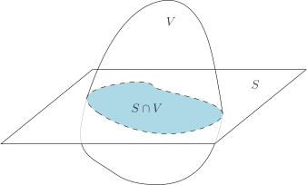
A three-dimensional volume \(V\) intersecting a charged surface \(S\).
To check \(\eqref{eq:charge_density_3d_from_2d}\), let
\(V\) be a volume that intersects \(S\) as in Figure 2. Then, \[\begin{aligned}
Q_V(t) &= \int_V\,\rho(t,\mathbf{x})\,d^3\mathbf{x}
=\int_S\left(\int_V
\delta(\mathbf{x}-\mathbf{x}(s_1,s_2))\,d^3\mathbf{x}\right)\sigma(t,s_1,s_2)\,dS\\
&=\int_{S\cap V}\sigma(t,s_1,s_2)\,dS= Q_{S\cap V}(t)\,,
\end{aligned}\] which is exactly what we expect from \(\eqref{eq:charge_density_surface}\). In
going from the first line to the second we used the basic property of
the delta function, namely that, \[\int_V
\delta(\mathbf{x}-\mathbf{x}(s_1,s_2))\,d^3\mathbf{x} = \begin{cases}
1& \mathrm{if}\,\mathbf{x}(s_1,s_2)\in V\\
0& \mathrm{if}\,\mathbf{x}(s_1,s_2)\notin V\,,
\end{cases}\] so the set of points contributing to the
integral is precisely \(S\cap V\).
As in the surface case, charge may also be confined to a
one-dimensional curve \(C\) with
parameter \(s\) and embedding \(\mathbf{x}(s)\). The linear charge density
\(\eta(t,s)\) is defined by, \[Q_{C'}(t)=\int_{C'}\eta(t,s)\,dl\,,\]
for a segment \(C' \subset C\),
where \(dl =
|\dot{\mathbf{x}}(s)|\,ds\). The associated three-dimensional
charge density is, \[\begin{equation}
\label{eq:charge_density_3d_from_1d}
\rho(t,\mathbf{x}) = \int_C \delta\left(\mathbf{x} -
\mathbf{x}(s)\right)\,\eta(t,s)\,dl\,. \end{equation}\]
For current densities, the geometry is slightly more delicate.
Consider a current \(I(t,s)\) flowing
along a curve \(C\) parameterised by
\(\mathbf{r}(s)\). From the
three-dimensional perspective, we would like a current density whose
flux through a surface \(S_p\) receives
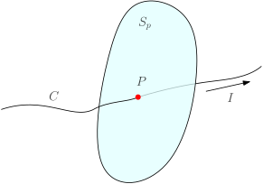
contributions only from the intersection points \(P=C\cap S_p\), as shown in Figure 3. As shown in Appendix 11, the correct expression is, \[\begin{align}
\label{eq:curr_density_curve}
\mathbf{J}(t,\mathbf{x})=\int_C
\delta(\mathbf{x}-\mathbf{r}(s))\,I(t,s)\,\dot{\mathbf{r}}(s)\,ds\,.
\end{align}\]
Intersection between a surface and a curve carrying
current.
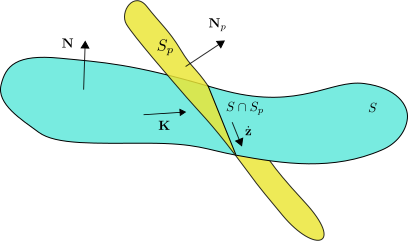
Finally, we consider a surface current density \(\mathbf{K}(t,\lambda_1,\lambda_2)\) flowing
on a surface \(S\) parameterised by
\(\mathbf{r}(\lambda_1,\lambda_2)\).
Since charge does not escape from the surface, \(\mathbf{K}\) is everywhere tangent to \(S\) and therefore orthogonal to the normal
vector \(\mathbf{N}=\partial_{\lambda_1}\mathbf{r}\times
\partial_{\lambda_2}\mathbf{r}\). From the perspective of the
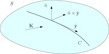
surface, it is natural to define the flux of current through a curve
\(C\) that lies entirely in \(S\), as shown in Figure 4. If \(C\subset S\) and \(\mathbf{y}(\lambda)=\mathbf{r}(\lambda_1(\lambda),\lambda_2(\lambda))\)
parameterises \(C\), then the tangent
vector \(\dot{\mathbf{y}}\) is
orthogonal2 to \(\mathbf{N}\).
Current flux through a curve.Flux of surface current through a transverse
surface.Current flux for surface current densities.
After defining the unit normal \(\hat{\mathbf{n}}\) to the surface, the
current flux across \(C\) can be
written as, \[\begin{align}
\label{eq:curr_flux_surf}
I_C(t)=\int_C
\mathbf{K}(t,\lambda_1(\lambda),\lambda_2(\lambda))\cdot\left(\hat{\mathbf{n}}\times
\dot{\mathbf{y}}(\lambda)\right)\,d\lambda\,.
\end{align}\] This mirrors the usual definition of flux through a
two-dimensional surface: here \(\hat{\mathbf{n}}\times \dot{\mathbf{y}}\)
plays the role of a normal “line element” along \(C\). Note that \(\hat{\mathbf{n}}\perp \dot{\mathbf{y}}\),
so \(\left|\hat{\mathbf{n}}\times
\dot{\mathbf{y}}\right|=\left|\dot{\mathbf{y}}\right|\).
From the three-dimensional perspective, we want a current density
whose flux through a surface \(S_p\)
reproduces the surface flux when \(S_p\) intersects \(S\) along the curve \(C=S\cap S_p\), as in Figure 6. As shown in Appendix 11, the appropriate distributional
current density is, \[\begin{align}
\label{eq:curr_density_surf}
\mathbf{J}(t,\mathbf{x})=\int_S
\delta\!\left(\mathbf{x}-\mathbf{r}(s_1,s_2)
\right)\,\mathbf{K}(t,s_1,s_2)\,dS\,,
\end{align}\] which indeed reduces to the correct expression when
integrated over \(S_p\).
3 Static
Fields
In the next few sections we will study charge and field
configurations that are time independent. For this to be
consistent, the charge and current densities sourcing the
electromagnetic field must have vanishing time derivatives. However,
charge and current density are not independent quantities. The charge
continuity equation \(\eqref{eq:charge_cont}\) implies that any
static current configuration must satisfy, \[\begin{align}
\label{eq:J_div}
\nabla\cdot\mathbf{J}=0\,.
\end{align}\]
Assuming we have somehow achieved such a steady flow of current,
Maxwell’s equations [eq:max_1,eq:max_2,eq:max_3,eq:max_4]
decouple the electric from the magnetic field into two separate sets. In
particular, the electric field is sourced purely by the charge
density,
These equations show that, in the absence of time dependence, one can
treat electric and magnetic fields as two largely independent entities.
Historically this is indeed how they were understood for a long time.
Allowing time dependence ties them together into a single theory,
electromagnetism, one of the first and most striking examples of
unification in physics.
Before studying these static systems in more detail, it is useful to
understand some general features that they share. Both are captured by a
set of differential equations of the form, \[\begin{align}
\nabla\cdot\mathbf{F}&=D\,,\notag\\
\nabla\times\mathbf{F}&=\mathbf{C}\,,\label{eq:f_system}
\end{align}\] for some given scalar field \(D\) and vector field \(\mathbf{C}\). Assuming \(\mathbf{F}\) is smooth, the second equation
implies the compatibility condition \(\nabla\cdot\mathbf{C}=0\), due to \(\eqref{eq:prop_1}\). For the electric field
this requirement is satisfied trivially because \(\eqref{eq:max_estatic_curl}\) sets \(\mathbf{C}=0\). For the magnetic field, on
the other hand, it becomes a non-trivial constraint. Taking the
divergence of \(\eqref{eq:max_bstatic_curl}\) requires
\(\nabla\cdot\mathbf{J}=0\), which is
precisely what the continuity equation enforces in a static
configuration.
A natural mathematical question is whether a system of equations like
\(\eqref{eq:f_system}\) is enough to
uniquely fix \(\mathbf{F}\). In
general, it is not. Indeed, given a solution \(\mathbf{F}_0\), we can always add to it a
vector field \(\mathbf{W}\) which
satisfies, \[\begin{aligned}
\nabla\cdot\mathbf{W}&=0\,,\\
\nabla\times\mathbf{W}&=0\,,
\end{aligned}\] and still obtain a solution with the same scalar
and vector sources. In fact, we can construct large families of such
fields by writing \(\mathbf{W}=\nabla
\phi\). Due to \(\eqref{eq:prop_2}\), the second equation is
then automatically satisfied, while the first reduces to the condition
that \(\phi\) is harmonic, \(\nabla^2\phi=0\). One such function is, for
example, \(\phi(x,y,z)=x\,y\,z\). The
ingredient we are missing in order to pin down a unique solution is
boundary conditions for the field \(\mathbf{F}\). We will not prove the general
statement here, since we will see explicitly how it works in the
following sections, when we discuss the scalar and vector
potentials.
If the divergence and the curl of a vector field \(\mathbf{F}\) are specified, and if they
both go to zero faster than \(1/r^2\)
at infinity and if \(\mathbf{F}\) goes
to zero as well, then \(\mathbf{F}\) is
uniquely fixed.
Illustration of superposition of static electric
fields.
Before moving on to examine our static configurations in more detail,
it is important to appreciate the linearity of the equations we are
dealing with. The linearity of Maxwell’s equations mirrors the
experimental observation that electric and magnetic fields satisfy a
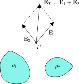
superposition principle. For example, consider the charge
distribution \(\rho_1\) sourcing the
electric field \(\mathbf{E}_1\) and the
charge distribution \(\rho_2\) sourcing
\(\mathbf{E}_2\). A highly non-obvious
fact is that when we put together the charge distributions to create the
total \(\rho_T=\rho_1+\rho_2\), the
resulting electric field is the vector sum \(\mathbf{E}_T=\mathbf{E}_1+\mathbf{E}_2\),
as illustrated in Figure 7.
Mathematically, this is reflected in the linearity of Maxwell’s
equations. Similar considerations apply for the magnetic field.
4
Electrostatics
In this section we focus on the electrostatic Maxwell equations \(\eqref{eq:max_estatic_div}\) and \(\eqref{eq:max_estatic_curl}\). We begin by
deriving the integral form of Gauss’ law, and then compute the
electric field for a number of charge distributions with simple
geometries. A particularly instructive example is an infinite plane with
uniform surface charge density. This system shows that surface charge
densities are naturally treated as discontinuities in the electric
field. We treat the more general case in the following subsection.
These examples help develop intuition for how an electric field is
sourced by a static charge distribution. More fundamentally, we
introduce the scalar potential and encounter the simplest form of gauge
symmetry. This also provides a convenient way to study the asymptotic
behaviour far from sources. Finally, we relate the work required to
assemble a charge distribution to the energy stored in the electric
field.
4.1
Gauss’ law
The first of Maxwell’s equations \(\eqref{eq:max_1}\) (or, in the
electrostatic case, \(\eqref{eq:max_estatic_div}\)) fixes the
divergence of the electric field. This is the differential form
of Gauss’ law. A great deal of intuition comes from integrating this
equation over a volume region \(V\),
\[\begin{aligned}
\int_V \nabla\cdot\mathbf{E}\,d^3\mathbf{x} =
\frac{1}{\varepsilon_0}\,\int_V \rho\,d^3\mathbf{x}\,.
\end{aligned}\] The integral on the right-hand side is simply the
total charge enclosed by \(V\), \[\begin{aligned}
Q_V \equiv \int_V \rho\,d^3\mathbf{x}\,.
\end{aligned}\] Applying Gauss’ theorem to the left-hand side
converts the volume integral into a surface integral over the closed
boundary \(S=\partial V\),
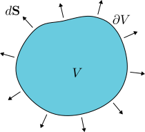
This is the integral form of Gauss’ law. When applying
Gauss’ theorem, the oriented area element \(d\mathbf{S}\) is defined using the
outward-pointing unit normal to \(\partial
V\), as illustrated in 8.
Orientation of boundary surface when applying Gauss’
theorem.
Electric field flux independent of surface
deformations.Gauss’ theorem illustrations.
Gauss’ law immediately constrains the net flux of \(\mathbf{E}\) through a closed surface. If
\(Q_V>0\), then the flux \(\int_{\partial V}\mathbf{E}\cdot
d\mathbf{S}\) is positive, so (on average) field lines exit the
surface. If \(Q_V<0\), the flux is
negative and the field lines enter the surface.
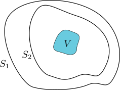
Gauss’ law also shows that the flux depends only on the charge
enclosed, not on the detailed shape of the surface. In particular, if we
deform \(\partial V\) continuously
without crossing any charge, the enclosed charge \(Q_V\) is unchanged and so is the flux. This
is illustrated in 10. Since the charge
density is non-zero only inside the volume \(V\), both surfaces \(S_1\) and \(S_2\) enclose the same charge, and
therefore the flux through either surface must be \(Q_V/\varepsilon_0\).
The remarks above are often enough to determine \(\mathbf{E}\) in situations with a high
degree of symmetry. In more general cases we will develop a more
systematic formalism (involving Green’s functions). Even in the
symmetric examples, however, one should keep in mind that Gauss’ law
\(\eqref{eq:gauss_law}\) is equivalent
only to \(\eqref{eq:max_estatic_div}\).
A full electrostatic solution must also satisfy \(\eqref{eq:max_estatic_curl}\) (together
with appropriate boundary conditions).
4.2 The
point particle - Coulomb’s law
In this section we study the electric field produced by a charged
point particle, the simplest electrostatic source one can consider. The
result is Coulomb’s law, which you have likely seen before, but it is
instructive to see how it follows directly from Maxwell’s equations.
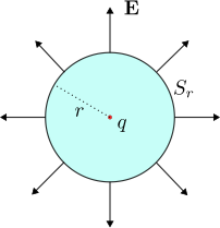
A sphere \(S_r\) of radius
\(r\) as a surface choice in Gauss’
law.
Given the spherical symmetry of the problem, the integral form of
Gauss’ law will be particularly useful for determining the electric
field. It is therefore natural to work in spherical coordinates \((r,\theta,\phi)\) with the corresponding
basis vectors \(\hat{\mathbf{e}}_r\),
\(\hat{\mathbf{e}}_\theta\) and \(\hat{\mathbf{e}}_\phi\). Assuming that the
charge sits at the origin, it is reasonable to expect that the electric
field has only a radial component, depending only on the radial
coordinate \(r\). More concretely, we
make the ansatz, \[\begin{align}
\label{eq:point_particle_ansatz}
\mathbf{E}(\mathbf{r}) = E(r)\,\hat{\mathbf{e}}_r\,,
\end{align}\] and then use Gauss’ law to determine the function
\(E(r)\). Note that this ansatz
satisfies \(\eqref{eq:max_estatic_curl}\) identically,
so we will not have to consider that equation further.
The natural choice of surface \(S\)
in Gauss’ law is a sphere \(S_r\) of
radius \(r\) centred at the origin,
where the point charge is located. In that case, \[\begin{aligned}
\int_{S_r}\mathbf{E}(\mathbf{r})\cdot
d\mathbf{S}=\frac{q}{\varepsilon_0}\,.
\end{aligned}\] To evaluate the integral, we note that the
oriented surface element is, \[\begin{aligned}
d\mathbf{S} =
\hat{\mathbf{e}}_r\,r^2\,\sin\theta\,d\theta\,d\phi=\hat{\mathbf{e}}_r\,r^2\,d\Omega\,,
\end{aligned}\] where \(d\Omega\) is the integration measure on the
unit sphere. The flux is therefore \[\begin{aligned}
\int_{S_r}\mathbf{E}(\mathbf{r})\cdot
d\mathbf{S}=\int_{S_r}E(r)\,r^2\,d\Omega=E(r)\,r^2\int_{S_r}d\Omega=4\pi\,E(r)\,r^2\,.
\end{aligned}\] Putting everything together, we find, \[\begin{aligned}
\mathbf{E}(\mathbf{r}) =
\frac{q}{4\pi\varepsilon_0}\,\frac{1}{r^2}\,\hat{\mathbf{e}}_r=\frac{q}{4\pi\varepsilon_0}\,\frac{\mathbf{r}}{r^3}\,,
\end{aligned}\] where we used that the position vector can always
be written as \(\mathbf{r}=r\,\hat{\mathbf{e}}_r\). If the
point charge is placed at \(\mathbf{r}_0\) instead of the origin, the
corresponding electric field is obtained by translation, \[\begin{align}
\label{eq:point_particle_E}
\mathbf{E}(\mathbf{r}) =
\frac{q}{4\pi\varepsilon_0}\,\frac{\mathbf{r}-\mathbf{r}_0}{\left|\mathbf{r}-\mathbf{r}_0\right|^3}\,,
\end{align}\] which is Coulomb’s law for the electric field of a
charged point particle.
While deriving \(\eqref{eq:point_particle_E}\) from the
integral form of Gauss’ law is satisfying, it is also useful to connect
back to the differential form \(\eqref{eq:max_estatic_div}\) and verify
that \(\eqref{eq:point_particle_E}\)
solves, \[\begin{aligned}
\nabla\cdot\mathbf{E}(\mathbf{r}) =
\frac{q}{\varepsilon_0}\,\delta(\mathbf{r}-\mathbf{r}_0)\,,
\end{aligned}\] since, according to Example [ex:point_particles_ch], the
charge density of a point particle is \(\rho(\mathbf{r})=q\,\delta(\mathbf{r}-\mathbf{r}_0)\).
4.3 The
infinite charged wire
The next geometry we examine is an infinite straight line \(C\) carrying a uniform linear charge
density \(\eta\). This configuration
has cylindrical symmetry because it is invariant under translations
along the line, a consequence of \(\eta\) being constant, and under rotations
about it. It is therefore natural to work in cylindrical coordinates
\((r,\phi,z)\) with basis vectors \(\hat{\mathbf{e}}_r\), \(\hat{\mathbf{e}}_\phi\) and \(\hat{\mathbf{e}}_z\), and to place the
charged line on the \(z\)-axis, i.e. at
\(r=0\). We note that if \(\eta\) depended on \(z\), the rotational symmetry would remain,
but translation invariance along the line would be lost.
By symmetry, the electric field must point radially and depend only
on the distance to the line. We therefore make the ansatz, \[\begin{aligned}
\mathbf{E}(\mathbf{r})=E(r)\,\hat{\mathbf{e}}_r\,,
\end{aligned}\] where “radial” is understood in the cylindrical
sense. As before, this ansatz satisfies \(\eqref{eq:max_estatic_curl}\) identically.
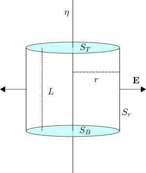
A convenient Gaussian surface is a cylinder \(S\) of length \(L\) and radius \(r\), coaxial with the line of charge, as
shown in Figure 12.
Gauss’ law applied to an infinite charged wire.
The charge enclosed by the cylinder comes entirely from the line, so
\(Q_V=\eta L\). The integral form of
Gauss’ law then gives, \[\begin{aligned}
\int_{S}\mathbf{E}(\mathbf{r})\cdot d\mathbf{S}=\frac{\eta
L}{\varepsilon_0}\,.
\end{aligned}\]
To evaluate the flux, decompose the surface as \(S=S_r\cup S_{T}\cup S_{B}\), where \(S_T\) and \(S_B\) are the top and bottom discs (of
radius \(r\)) and \(S_r\) is the cylindrical side. The end caps
do not contribute, since their outward normal is parallel to \(\hat{\mathbf{e}}_z\), which is orthogonal
to \(\mathbf{E}\). For the side surface
we use, \[\begin{aligned}
d\mathbf{S}_r = \hat{\mathbf{e}}_r\,r\,d\phi\,dz\,,
\end{aligned}\] and hence, \[\begin{aligned}
\int_{S}\mathbf{E}(\mathbf{r})\cdot
d\mathbf{S}=\int_{S_r}\mathbf{E}(\mathbf{r})\cdot
d\mathbf{S}_r=r\,E(r)\,\int_{0}^{2\pi}\int_{0}^{L}dz\,d\phi=2\pi\,L\,r\,E(r)\,.
\end{aligned}\] Combining these results, we obtain the electric
field of an infinite charged wire, \[\begin{aligned}
\mathbf{E}(\mathbf{r})=\frac{\eta}{2\pi\varepsilon_0}\,\frac{1}{r}\,\hat{\mathbf{e}}_r\,.
\end{aligned}\]
4.4 The
infinite charged surface
The final highly symmetric geometry we will examine is an infinite
plane carrying a uniform surface charge density \(\sigma\). The relevant symmetries are
translations in the two directions parallel to the plane. A convenient
coordinate system is therefore Cartesian coordinates \((x,y,z)\) with basis vectors \(\hat{\mathbf{e}}_x\), \(\hat{\mathbf{e}}_y\) and \(\hat{\mathbf{e}}_z\).
The symmetry of the configuration suggests that the electric field is
everywhere normal to the plane, which we take to lie at \(z=0\). Moreover, reflecting the system
through the plane sends \(z\to -z\)
while leaving the charge distribution unchanged; since the electric
field is a vector, it must transform as \(\mathbf{E}(-z)=-\mathbf{E}(z)\). A natural
ansatz consistent with these symmetries is, \[\begin{align}
\label{eq:infinite_plane_ansatz}
\mathbf{E}(z)=\begin{cases}
E(z)\,\hat{\mathbf{e}}_z&\mathrm{if}\, z>0\,,\\
-E(-z)\,\hat{\mathbf{e}}_z&\mathrm{if}\, z<0\,.
\end{cases}
\end{align}\] It is straightforward to check that \(\eqref{eq:max_estatic_curl}\) is satisfied
identically by construction.
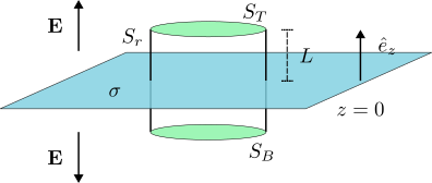
Electric field generated by a uniformly charged infinite
plane.
A natural Gaussian surface for this geometry is a cylinder \(S\) whose axis is perpendicular to the
charged plane and whose midpoint lies at \(z=0\). Choosing the cylinder to have total
length \(2L\), its two bases \(S_T\) and \(S_B\) (each of area \(A\)) are located at \(z=L\) and \(z=-L\), respectively We have included 13 for illustration.
The intersection of the cylinder with the charged plane is a disk of
area \(A\), so the total enclosed
charge comes entirely from this disk and equals \(Q_V=\sigma A\). Gauss’ law therefore gives,
\[\begin{aligned}
\int_S \mathbf{E}\cdot d\mathbf{S}= \frac{\sigma
A}{\varepsilon_0}\,.
\end{aligned}\] We decompose the flux as, \[\begin{aligned}
\int_S \mathbf{E}\cdot d\mathbf{S}=\int_{S_r} \mathbf{E}\cdot
d\mathbf{S_r}+\int_{S_T} \mathbf{E}\cdot d\mathbf{S_T}+\int_{S_B}
\mathbf{E}\cdot d\mathbf{S_B}\,,
\end{aligned}\] where \(S_r\)
denotes the cylindrical side surface. The first term vanishes because
\(\mathbf{E}\) is parallel to the
cylinder axis, whereas \(d\mathbf{S}_r\) is orthogonal to it. Taking
the outward orientation into account, the oriented area elements on the
two bases are, \[\begin{aligned}
d\mathbf{S_T}&= \hat{\mathbf{e}}_z\,dS_T\,,\\
d\mathbf{S_B}&= -\hat{\mathbf{e}}_z\,dS_B\,.
\end{aligned}\] The corresponding surface integrals are, \[\begin{aligned}
\int_{S_T} \mathbf{E}\cdot
d\mathbf{S_T}&=\int_{S_T}\mathbf{E}(z=L)\cdot\hat{\mathbf{e}}_z\,dS_T=E(L)\,\int_{S_T}dS_T=E(L)\,A\,,\\
\int_{S_B} \mathbf{E}\cdot
d\mathbf{S_B}&=-\int_{S_B}\mathbf{E}(z=-L)\cdot\hat{\mathbf{e}}_z\,dS_B=E(L)\,\int_{S_B}dS_B=E(L)\,A\,.
\end{aligned}\] Putting everything together fixes the function in
the ansatz \(\eqref{eq:infinite_plane_ansatz}\) to be a
constant, \[\begin{aligned}
E(z)=\frac{\sigma}{2\varepsilon_0}\,.
\end{aligned}\] The fact that the electric field is constant for
\(z\neq 0\) is far from obvious until
one applies Gauss’ law.
A key point is what happens at the location of the charged plane
itself. The solution \(\eqref{eq:infinite_plane_ansatz}\) implies
the jump condition, \[\begin{align}
\label{eq:infinite_plane_disctontinuity}
\mathbf{E}(z=0^+)-\mathbf{E}(z=0^-)=\frac{\sigma}{\varepsilon_0}\,\hat{\mathbf{e}}_z\Rightarrow
\left.\begin{array}{l}
\hat{\mathbf{e}}_z\cdot\left(\mathbf{E}(z=0^+)-\mathbf{E}(z=0^-)\right)=\frac{\sigma}{\varepsilon_0}\,,\\
\hat{\mathbf{e}}_z\times\left(\mathbf{E}(z=0^+)-\mathbf{E}(z=0^-)\right)=0
\end{array}\right\}\,.
\end{align}\] This shows that the component normal to the surface
is discontinuous, with a jump fixed by the surface charge density. The
second equation states that any tangential component would be
continuous; in the present example it is trivially satisfied since the
field is everywhere normal to the plane.
It is instructive to see why this discontinuity is unavoidable
directly from the differential form of Gauss’ law \(\eqref{eq:max_estatic_div}\). Since
symmetry implies \(\mathbf{E}=E_z(z)\,\hat{\mathbf{e}}_z\),
equation \(\eqref{eq:max_estatic_div}\)
becomes, \[\begin{aligned}
\partial_z E_z(z)=\frac{1}{\varepsilon_0}\,\rho(x,y,z)\,,
\end{aligned}\] with \(\rho\)
the three-dimensional charge density. Using \(\eqref{eq:charge_density_3d_from_2d}\) with
the surface parametrisation \(\mathbf{x}(s_1,s_2)=(s_1,s_2,0)\), we find,
\[\begin{aligned}
\rho(x,y,z)&=\int_{\mathbb{R}^2}\sigma\,\delta(x-s_1)\,\delta(y-s_2)\,\delta(z)\,ds_1\,ds_2\\
&=\sigma\,\delta(z)\,\int_{\mathbb{R}^2}\delta(x-s_1)\,\delta(y-s_2)\,ds_1\,ds_2\\
&=\sigma\,\delta(z)\,,
\end{aligned}\] as expected. The charge density is proportional
to a delta function supported at the surface. Gauss’ law therefore takes
the form, \[\begin{aligned}
\partial_z E_z(z)=\frac{\sigma}{\varepsilon_0}\,\delta(z)\,.
\end{aligned}\] Integrating from \(z=-\epsilon\) to \(z=\epsilon\) gives precisely the
discontinuity already obtained above, \[\begin{aligned}
\int_{-\epsilon}^\epsilon \partial_z
E_z(z)\,dz=\frac{\sigma}{\varepsilon_0}\,\int_{-\epsilon}^\epsilon
\delta(z)\,dz\Rightarrow
E_z(\epsilon)-E_z(-\epsilon)=\frac{\sigma}{\varepsilon_0}\,.
\end{aligned}\] In evaluating the integral on the right-hand side
we used the defining property of the Dirac delta, discussed in Appendix
10.
This argument shows that such jump conditions are far more general
than the flat surface considered here. In the next section we discuss
the general case; the underlying idea is the same as in this
example.
4.5
Surface Charge as an Interface
This subsection is non-examinable.
In the previous section we studied the electric field generated by an
infinite plane carrying a uniform surface charge density. The key lesson
was that the component of \(\mathbf{E}\) normal to the surface is
discontinuous. We traced this discontinuity back to the Dirac delta
appearing in \(\eqref{eq:charge_density_3d_from_2d}\),
which relates the surface charge density \(\sigma\) to the three-dimensional charge
density \(\rho\). Here we derive the
corresponding jump conditions for a general surface \(S\) carrying a surface charge density \(\sigma\), which may vary along the surface
and, more generally, in time.
Integration over a Gaussian surface.
Integration over a loop.Surface and loop integrations used to derive boundary
conditions for the electric field.
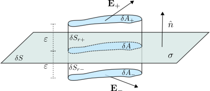
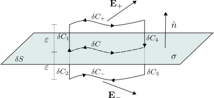
To study the discontinuity of the component of \(\mathbf{E}\) normal to \(S\), we use a pillbox-type Gaussian surface
adapted to an arbitrary patch of the interface. Consider a small section
\(\delta S\subset S\) with unit normal
vector \(\hat{\mathbf{n}}\), as shown
in Figure 14. For ease of
illustration the patch is drawn as flat, but the argument does not rely
on this.
To construct the Gaussian surface, choose a small area \(\delta A\subset \delta S\) and extrude each
point of \(\delta A\) by \(\varepsilon\) along \(\hat{\mathbf{n}}\). The collection of all
resulting trajectories forms a (generalised) cylinder \(V_+\) with bases \(\delta A\) and \(\delta {A_+}\), and side \(\delta S_+\). Repeating the construction by
extruding \(\delta A\) in the opposite
direction produces a second cylinder \(V_-\) with bases \(\delta A\) and \(\delta {A_-}\), and side \(\delta S_-\).
Gauss’ law for the volume \(V=V_+\cup
V_-\) reads, \[\begin{aligned}
\int_{\partial V}\mathbf{E}\cdot d\mathbf{S} =
\frac{1}{\varepsilon_0} Q_{V}\,,
\end{aligned}\] where \(\partial
V\) is the boundary of \(V\).
The only charge inside \(V\) comes from
the surface charge contained in \(\delta
A\), so, \[\begin{aligned}
Q_V = \int_{\delta A} \sigma\,dS\,.
\end{aligned}\] The flux of the electric field can be decomposed
as, \[\begin{align}
\label{eq:surface_discontinuity_flux}
\int_{\partial V}\mathbf{E}\cdot d\mathbf{S} = \int_{\delta
A_+}\mathbf{E}\cdot d\mathbf{S} + \int_{\delta S_+}\mathbf{E}\cdot
d\mathbf{S}+ \int_{\delta A_-}\mathbf{E}\cdot d\mathbf{S} + \int_{\delta
S_-}\mathbf{E}\cdot d\mathbf{S}\,.
\end{align}\] Remark [rem:surface_deform] suggests
that this flux should be independent of \(\varepsilon\), including in the \(\varepsilon\to 0\) limit. By construction,
the charge \(Q_V\) is also independent
of \(\varepsilon\).
To evaluate the flux in this limit, note that the side surfaces \(\delta S_+\) and \(\delta S_-\) shrink to zero area as \(\varepsilon\to 0\). Provided the electric
field remains finite (as we expect in the absence of further singular
sources), the second and fourth terms in \(\eqref{eq:surface_discontinuity_flux}\)
therefore vanish. In the same limit, both bases \(\delta A_+\) and \(\delta A_-\) converge to \(\delta A\), with orientations \(\hat{\mathbf{n}}\) and \(-\hat{\mathbf{n}}\), respectively. It
follows that, \[\begin{aligned}
\lim_{\varepsilon\to 0^+}\int_{\delta A_+}\mathbf{E}\cdot
d\mathbf{S} &= \int_{\delta A}\hat{\mathbf{n}}\cdot\mathbf{E}_{+}
\,dS\,,\notag\\
\lim_{\varepsilon\to 0^+}\int_{\delta A_-}\mathbf{E}\cdot
d\mathbf{S} &= -\int_{\delta A}\hat{\mathbf{n}}\cdot\mathbf{E}_{-}
\,dS\,,
\end{aligned}\] where \(\mathbf{E}_{+}\) is the limit of the
electric field as we approach \(\delta
S\) from the side toward which \(\hat{\mathbf{n}}\) points, and \(\mathbf{E}_{-}\) is the corresponding limit
from the opposite side.
Putting everything together, and using that \(\delta A\) was arbitrary, Gauss’ law \(\eqref{eq:surface_discontinuity_flux}\)
yields the discontinuity condition,
Beyond the normal component, we would also like to understand what
happens to the components of \(\mathbf{E}\) tangent to the surface. In the
planar example these components vanished by symmetry and were therefore
trivially continuous. In the general case we need an argument that does
not rely on symmetry.
Instead of an area \(\delta A\),
consider a curve \(\delta C\) lying
within the surface \(\delta S\).
Repeating the extrusion construction along the unit normal \(\hat{\mathbf{n}}\) produces a surface \(\delta S_l\) bounded by the loop \(\delta C_l=\delta C_1\cup \delta C_2\cup \delta
C_-\cup \delta C_3\cup \delta C_4 \cup \delta C_+\), as shown in
Figure 16. Integrating both
sides of \(\eqref{eq:max_estatic_curl}\) over \(\delta S_l\) and applying Stokes’ theorem
gives, \[\begin{aligned}
&\int_{\delta S_l}\left(\nabla\times\mathbf{E}\right)\cdot
d\mathbf{S}=0\Rightarrow\notag\\
&\int_{\delta C_l}\mathbf{E}\cdot
d\mathbf{r}=0\notag\Rightarrow\\
&\int_{\delta C_1}\mathbf{E}\cdot d\mathbf{l}+\int_{\delta
C_2}\mathbf{E}\cdot d\mathbf{l}+\int_{\delta C_-}\mathbf{E}\cdot
d\mathbf{l}+\int_{\delta C_3}\mathbf{E}\cdot d\mathbf{l}+\int_{\delta
C_4}\mathbf{E}\cdot d\mathbf{l}+\int_{\delta C_+}\mathbf{E}\cdot
d\mathbf{l}=0\,,
\end{aligned}\] with orientations as in Figure 16. Taking the \(\varepsilon\to 0\) limit, the segments
\(\delta C_i\) for \(i=1,\ldots,4\) shrink to zero and their
contributions vanish. In the same limit, \(\delta C_+\) and \(\delta C_-\) both approach the curve \(\delta C\) with opposite orientations, and
we obtain, \[\begin{aligned}
\int_{\delta C}\left(\mathbf{E}_+-\mathbf{E}_- \right)\cdot
d\mathbf{r}=0\,.
\end{aligned}\] Since this holds for any curve \(\delta C\subset \delta S\), we can also
write the local condition, \[\begin{aligned}
\hat{\mathbf{n}}_{\parallel}\cdot\left(\mathbf{E}_+-\mathbf{E}_-
\right)=0\,,
\end{aligned}\] for any vector \(\hat{\mathbf{n}}_{\parallel}\) tangent to
the surface \(\delta S\). An
equivalent, and often more practical, way of expressing this condition
is in terms of the unit normal,
We have therefore shown that the component of the electric field
parallel to the surface is continuous.
4.6 The
Electrostatic Potential
So far we have been able to determine the electric field in a number
of highly symmetric electrostatic setups. In each case we could write
down an ansatz for \(\mathbf{E}\) that
automatically satisfied the curl-free condition \(\eqref{eq:max_estatic_curl}\). It is worth
pausing to understand what this equation implies more generally.
By Stokes’ theorem, \(\eqref{eq:max_estatic_curl}\) implies that
the line integral of the electric field around any closed loop \(C\) vanishes,
Equivalently, the line integral of \(\mathbf{E}\) along a curve connecting two
fixed endpoints \(\mathbf{r}_1\) and
\(\mathbf{r}_2\) depends only on the
endpoints and not on the particular path. Since the force on a particle
of charge \(q\) is \(\mathbf{F}=q\,\mathbf{E}\), this means that
the work, \[\begin{aligned}
W_{12} = \int_{C_{12}} \mathbf{F}\cdot d\mathbf{r}
=q\,\int_{C_{12}} \mathbf{E}\cdot d\mathbf{r}
\end{aligned}\] required to move the particle from \(\mathbf{r}_1\) to \(\mathbf{r}_2\) along any path \(C_{12}\) is path independent.
In addition, the identity \(\eqref{eq:prop_2}\) shows that \(\eqref{eq:max_estatic_curl}\) is
automatically satisfied if we write the electric field as a
gradient,
for some scalar function \(\varphi\), called the scalar (or
electrostatic) potential. In fact, one can prove the converse
as well. Under appropriate regularity assumptions, any curl-free field
can be written locally in this form. Substituting \(\eqref{eq:scalar_potential}\) into Gauss’
law \(\eqref{eq:max_estatic_div}\)
gives a single scalar equation for \(\varphi\),
which is often considerably simpler to analyse than the original
coupled system.
We should now make the following remarks,
The physically relevant quantity is the electric field \(\mathbf{E}\), not the potential \(\varphi\). Notice that \(\mathbf{E}\) is invariant under shifts of
\(\varphi\) by a constant. We usually
fix this constant by choosing a convention, for example by demanding
that \(\varphi\) vanishes at infinity
(when this is compatible with the physical setup).
For a particle of charge \(q\)
moving in an electric field \(\mathbf{E}\), the potential energy is \(V(\mathbf{x})=q\,\varphi(\mathbf{x})\). The
corresponding Lagrangian is, \[\begin{aligned}
L=\frac{1}{2}m\,\dot{\mathbf{x}}^2-q\,\varphi(\mathbf{x})\,.
\end{aligned}\]
With the boundary condition that \(\mathbf{E}\) vanishes at infinity, the
equation for \(\varphi\) is linear and
the potential obeys a superposition principle. If \(\rho=\rho_1+\rho_2\), then (after fixing
the same reference for the additive constant) \(\varphi=\varphi_1+\varphi_2\).
At this point we can appreciate that introducing the scalar potential
is a very useful way to simplify Maxwell’s equations. However, as we
will later see, it has a more fundamental meaning than a mere
computational trick. Moreover, Remark [rem:electrostatic_gauge_symmetry]
is the simplest example of what we will later call a gauge
symmetry.
We now consider an instructive example of solving \(\eqref{eq:electrostatic_spontential_eq}\)
for a point charge.
We solve \(\eqref{eq:electrostatic_spontential_eq}\)
for a particle carrying electric charge \(q\). If the particle is at rest at the
origin, Example [ex:point_particles_ch] gives
the charge density \(\rho(\mathbf{x})=q\,\delta(\mathbf{x})\),
and the potential must satisfy, \[\begin{align}
\label{eq:point_particle_potential_eq}
\nabla^2
\varphi(\mathbf{x})=-\frac{q}{\varepsilon_0}\,\delta(\mathbf{x})\,.
\end{align}\] Spherical symmetry suggests using spherical
coordinates, with \(\varphi\) depending
only on the radial coordinate \(r\).
We first solve the equation away from the origin, where the
delta-function source vanishes. In this region we have, \[\begin{aligned}
\frac{1}{r^2}\partial_r\left(r^2\,\partial_r\varphi(r)\right)=0\,.
\end{aligned}\] whose general solution is, \[\begin{aligned}
\varphi(r)=\frac{a}{r}+b\,,
\end{aligned}\] with constants of integration \(a\) and \(b\). Following Remark [rem:electrostatic_gauge_symmetry]
and choosing \(\varphi\to 0\) as \(r\to\infty\) fixes \(b=0\). The remaining constant \(a\) is determined by requiring that \(\eqref{eq:point_particle_potential_eq}\)
holds globally, including at the origin.
To do this, integrate both sides of \(\eqref{eq:point_particle_potential_eq}\)
over a ball \(B_R\) of radius \(R\). The integral of the right-hand side is
\(-q/\varepsilon_0\), since the origin
lies inside \(B_R\). For the left-hand
side we use Gauss’ theorem to convert the volume integral over \(B_R\) into a surface integral over the
sphere \(S_R\) of radius \(R\). Since \(\nabla\varphi
=-\frac{a}{r^2}\,\hat{\mathbf{e}}_r\), we find, \[\begin{aligned}
\int_{B_R}\nabla^2\varphi\,d^3\mathbf{x}
=\int_{S_R}\nabla\varphi\cdot d\mathbf{S}
=-\frac{a}{R^2}\int_{S_R}\hat{\mathbf{e}}_r\cdot d\mathbf{S}
=-\frac{a}{R^2}\,R^2\int_{S_R}d\Omega
=-4\pi a\,.
\end{aligned}\] Here we used \(d\mathbf{S}=R^2\,\hat{\mathbf{e}}_r\,d\Omega\),
where \(d\Omega\) is the area element
on the unit sphere. Equating both sides gives \(a=\frac{q}{4\pi\varepsilon_0}\), and
therefore, \[\begin{aligned}
\varphi(\mathbf{x})=\frac{q}{4\pi\varepsilon_0}\,\frac{1}{|\mathbf{x}|}\,.
\end{aligned}\] If the particle is located at \(\mathbf{x}_0\) instead of the origin, the
equation becomes, \[\begin{align}
\label{eq:point_particle_potential_eq_2}
\nabla^2
\varphi(\mathbf{x})=-\frac{q}{\varepsilon_0}\,\delta(\mathbf{x}-\mathbf{x}_0)\,,
\end{align}\] and by translation invariance we obtain, \[\begin{align}
\label{eq:point_particle_potential}
\varphi(\mathbf{x})=\frac{q}{4\pi\varepsilon_0}\,\frac{1}{|\mathbf{x}-\mathbf{x}_0|}\,.
\end{align}\] The resulting electric field is, \[\begin{aligned}
\mathbf{E}(\mathbf{x})=-\nabla\varphi(\mathbf{x})
=-\frac{q}{4\pi\varepsilon_0}\,\nabla\left(\frac{1}{|\mathbf{x}-\mathbf{x}_0|}\right)
=\frac{q}{4\pi\varepsilon_0}\,\frac{\mathbf{x}-\mathbf{x}_0}{|\mathbf{x}-\mathbf{x}_0|^3}\,,
\end{aligned}\] in agreement with \(\eqref{eq:point_particle_E}\).
4.7 The
General Charge Density
In Example [ex:point_particle_spotential]
of the previous section we solved a seemingly simple problem. As we will
see in this section, that calculation contains the basic ingredient
needed to write down the solution for a general charge density \(\rho(\mathbf{x})\). At a technical level,
equations \(\eqref{eq:point_particle_potential_eq_2}\)
and \(\eqref{eq:point_particle_potential}\) tell
us that we have found a function,
A function \(G(\mathbf{x},\mathbf{x}_0)\) satisfying
\(\eqref{eq:greens_function_def}\) is
important enough to have its own name, it is a Green’s function
for the Laplace operator.
Given a charge distribution \(\rho(\mathbf{x})\) that decays
“sufficiently fast” at infinity, the scalar potential \(\varphi(\mathbf{x})\) solving \(\eqref{eq:electrostatic_spontential_eq}\)
is,
The fall-off condition ensures that the integral converges and, for
this choice of \(G\), that \(\varphi\) vanishes at infinity.
To check that \(\eqref{eq:scalar_potential_general_sol}\)
indeed solves \(\eqref{eq:electrostatic_spontential_eq}\),
we apply the Laplace operator with respect to \(\mathbf{x}\), \[\begin{aligned}
\nabla^2\varphi(\mathbf{x})=&-\frac{1}{\varepsilon_0}\,\nabla^2\left(\int
\rho(\mathbf{x}^\prime)\,G(\mathbf{x},\mathbf{x}^\prime)\,d^3\mathbf{x}^\prime\right)\notag\\
=&-\frac{1}{\varepsilon_0}\,\int
\rho(\mathbf{x}^\prime)\,\nabla^2
G(\mathbf{x},\mathbf{x}^\prime)\,d^3\mathbf{x}^\prime\notag\\
=&-\frac{1}{\varepsilon_0}\,\int
\rho(\mathbf{x}^\prime)\,\delta(\mathbf{x}-\mathbf{x}^\prime)\,d^3\mathbf{x}^\prime=-\frac{1}{\varepsilon_0}\,\rho(\mathbf{x})\,.
\end{aligned}\] From the second line to the third we used the
defining property \(\eqref{eq:greens_function_def}\) of the
Green’s function; in the last step we used the defining property of the
Dirac delta.
Given the solution \(\eqref{eq:scalar_potential_general_sol}\)
for the scalar potential, we can compute the electric field as,
It is striking that a single function \(G\) yields the solution for an arbitrary
source. From a physicist’s point of view, however, the structure of
\(\eqref{eq:electric_field_general_sol}\) is
also natural. It is precisely a continuous version of the superposition
of point-charge fields in \(\eqref{eq:point_particle_E}\).
We now apply the general result for the scalar potential to the
configuration of \(N\) stationary point
charges from Example [ex:point_particles_ch]. The
charge density is, \[\begin{aligned}
\rho\left(\mathbf{x}^\prime\right)=\sum_{i=1}^N
q_i\,\delta\left(\mathbf{x}^\prime - \mathbf{y}_i\right)\,.
\end{aligned}\] Substituting this into \(\eqref{eq:scalar_potential_general_sol}\)
gives, \[\begin{aligned}
\varphi(\mathbf{x})&=\frac{1}{4\pi\varepsilon_0}\,\int \left(
\sum_{i=1}^N q_i\,\delta\left(\mathbf{x}^\prime -
\mathbf{y}_i\right)\right)\frac{1}{|\mathbf{x}-\mathbf{x}^\prime|}\,d^3\mathbf{x}^\prime\notag\\
&=\frac{1}{4\pi\varepsilon_0}\, \sum_{i=1}^N
q_i\,\int\frac{\delta\left(\mathbf{x}^\prime -
\mathbf{y}_i\right)}{|\mathbf{x}-\mathbf{x}^\prime|}\,d^3\mathbf{x}^\prime\notag\\
&=\frac{1}{4\pi\varepsilon_0}\, \sum_{i=1}^N
\frac{q_i}{|\mathbf{x}-\mathbf{y}_i|}\,,
\end{aligned}\] which, as expected, is a simple superposition of
the single-particle result \(\eqref{eq:point_particle_potential}\). The
corresponding electric field is, \[\begin{aligned}
\mathbf{E}(\mathbf{x})=-\nabla\varphi(\mathbf{x})=\frac{1}{4\pi\varepsilon_0}\, \sum_{i=1}^N
q_i\,\frac{\mathbf{x}-\mathbf{y}_i}{|\mathbf{x}-\mathbf{y}_i|^3}\,,
\end{aligned}\] which can also be obtained directly from \(\eqref{eq:electric_field_general_sol}\) by
evaluating the integral for this charge density.
There is an important subtlety regarding the Green’s function. The
defining equation \(\eqref{eq:greens_function_def}\) must be
supplemented with boundary conditions in order to determine \(G(\mathbf{x},\mathbf{x}_0)\) uniquely. The
expression \(\eqref{eq:greens_function}\) corresponds to
boundary conditions where the potential vanishes at infinity. Indeed,
taking \(|\mathbf{x}|\) large in the
second line of \(\eqref{eq:scalar_potential_general_sol}\)
gives \(\varphi(\mathbf{x})\to 0\) as
\(|\mathbf{x}|\to\infty\).
There is a class of important problems involving conducting surfaces
\(S\), where one instead imposes \(\varphi=0\) on \(S\). When \(S\) is not at infinity, the Green’s
function differs from \(\eqref{eq:greens_function}\). The general
solution is still given by the first line of \(\eqref{eq:scalar_potential_general_sol}\),
but with the Green’s function appropriate to the chosen boundary
conditions.
Before closing this section, we will write the general solutions for
the scalar potential for the cases of surface and linear charge
densities. In fact, we can plug in the expressions \(\eqref{eq:charge_density_3d_from_2d}\) and
\(\eqref{eq:charge_density_3d_from_1d}\) in
the solution \(\eqref{eq:scalar_potential_general_sol}\)
to obtain, \[\begin{aligned}
\varphi(\mathbf{x})&=\frac{1}{4\pi\,\varepsilon_0}\int_S
\frac{\sigma(s_1,s_2)}{\left|\mathbf{x}-\mathbf{x}^\prime(s_1,s_2)\right|}\,dS\,,\\
\varphi(\mathbf{x})&=\frac{1}{4\pi\,\varepsilon_0}\int_C
\frac{\eta(s)}{\left|\mathbf{x}-\mathbf{x}^\prime(s_1,s_2)\right|}\,dl\,.
\end{aligned}\] with electric fields, \[\begin{aligned}
\mathbf{E}(\mathbf{x})&=\frac{1}{4\pi\,\varepsilon_0}\int_S
\sigma(s_1,s_2)\,\frac{\mathbf{x}-\mathbf{x}^\prime(s_1,s_2)}{\left|\mathbf{x}-\mathbf{x}^\prime(s_1,s_2)\right|^3}\,dS\,,\\
\mathbf{E}(\mathbf{x})&=\frac{1}{4\pi\,\varepsilon_0}\int_C
\eta(s)\,\frac{\mathbf{x}-\mathbf{x}^\prime(s_1,s_2)}{\left|\mathbf{x}-\mathbf{x}^\prime(s_1,s_2)\right|^3}\,dl\,.
\end{aligned}\]
4.8 The
Multipole Expansion (Long Distance Behaviour)
In this section we study the scalar potential and electric field far
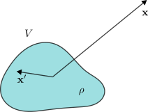
from their sources, as illustrated in Figure 17. We assume that the charge
density \(\rho(\mathbf{x})\) is
localised inside a bounded region \(V\subset\mathbb{R}^3\), so \(\rho(\mathbf{x})=0\) outside \(V\). In the integral expression \(\eqref{eq:scalar_potential_general_sol}\),
the integration variable \(\mathbf{x}^\prime\) therefore ranges only
over \(V\). We are interested in the
behaviour of the potential at observation points satisfying \(|\mathbf{x}|\gg |\mathbf{x}^\prime|\) for
all \(\mathbf{x}^\prime\in V\).
Behaviour at distances far away from the
sources.
The key ingredient is an asymptotic expansion of the Green’s-function
kernel, \[\begin{align}
\frac{1}{|\mathbf{x}-\mathbf{x}^\prime|}&=\frac{1}{|\mathbf{x}|}-\mathbf{x}^\prime\cdot\nabla
\frac{1}{|\mathbf{x}|}+\frac{1}{2}\left(\mathbf{x}^\prime\cdot\nabla\right)^2\frac{1}{|\mathbf{x}|}+\cdots\notag\\
&=\frac{1}{|\mathbf{x}|}+\frac{\mathbf{x}\cdot
\mathbf{x}^\prime}{|\mathbf{x}|^3}+\cdots\,,\label{eq:large_distance_exp}
\end{align}\] which is simply the Taylor expansion in \(\mathbf{x}^\prime\), with derivatives
acting on \(\mathbf{x}\). Keeping only
the first few terms and substituting into the general solution \(\eqref{eq:scalar_potential_general_sol}\)
gives, \[\begin{align}
\varphi(\mathbf{x})&=\frac{1}{4\pi\varepsilon_0}\frac{1}{|\mathbf{x}|}\,\int_V\rho(\mathbf{x}^\prime)\,d^3\mathbf{x}^\prime
+\frac{1}{4\pi\varepsilon_0}\frac{1}{|\mathbf{x}|^3}\,\mathbf{x}\,\cdot\int_V\rho(\mathbf{x}^\prime)\,\mathbf{x}^\prime\,d^3\mathbf{x}^\prime+\cdots\notag\\
&=\frac{1}{4\pi\varepsilon_0}\frac{Q}{|\mathbf{x}|}
+\frac{1}{4\pi\varepsilon_0}\frac{\mathbf{x}\cdot
\mathbf{p}}{|\mathbf{x}|^3}+\cdots\,.\label{eq:large_distance_exp_scalar_potential}
\end{align}\] In this expansion we have defined,
as the total charge (the monopole moment) and the dipole
moment of the charge distribution. Keeping higher-order terms in
\(\eqref{eq:large_distance_exp}\) would
similarly define higher multipole moments. The general pattern is that
higher moments contribute terms that fall off more rapidly far from the
sources. The monopole potential scales as \(1/|\mathbf{x}|\), while the dipole
correction scales as \(1/|\mathbf{x}|^2\).
The corresponding electric field is obtained by taking the
gradient,
The first term is the Coulomb field produced by the total charge
\(Q\), while the second is the leading
correction due to the dipole moment.
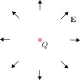
Electric field with \(Q\neq
0\) and \(\mathbf{p}=0\).
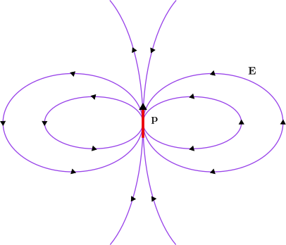
Electric field with \(Q=
0\) and \(\mathbf{p}\neq
0\).Field lines of distributions with different dominant
moments.
Based on this general discussion, we can make the following
remarks,
From the expansion \(\eqref{eq:large_distance_exp_scalar_potential}\),
an observer far away from the sources first measures the net charge
\(Q\) of the distribution. When \(Q\neq 0\), the dipole moment \(\mathbf{p}\) appears as a subleading
distortion of the spherically symmetric monopole field.
The dipole moment depends on the choice of origin (and the same is
true for all higher moments). In fact, under a translation of the
coordinate system by \(\mathbf{a}\),
one finds \(\mathbf{p}\mapsto
\mathbf{p}+Q\,\mathbf{a}\). In particular, for a spherically
symmetric charge distribution, choosing the origin at the centre of
symmetry sets all multipole moments beyond \(Q\) to zero.
There are charge distributions for which either \(Q\) or \(\mathbf{p}\) vanishes. The corresponding
electric fields are illustrated in Figures 18 and 20.
It is instructive to work out the moments explicitly for a simple
example involving two particles,
We consider two point charges \(q_1\) and \(q_2\) located at positions \(\mathbf{x}_1\) and \(\mathbf{x}_2\) in a chosen coordinate
system.
The coordinate-independent quantity is their relative displacement
\(\mathbf{d}=\mathbf{x}_1-\mathbf{x}_2\). The
charge density is, \[\begin{aligned}
\rho(\mathbf{x})=q_1\,\delta(\mathbf{x}-\mathbf{x}_1)+
q_2\,\delta(\mathbf{x}-\mathbf{x}_2)\,.
\end{aligned}\] The total charge is, \[\begin{aligned}
Q&=\int
\rho(\mathbf{x})\,d^3\mathbf{x}=q_1\,\int\delta(\mathbf{x}-\mathbf{x}_1)\,d^3\mathbf{x}+q_2\,\int\delta(\mathbf{x}-\mathbf{x}_2)\,d^3\mathbf{x}\notag\\
&=q_1+q_2\,,
\end{aligned}\] as expected. The dipole moment \(\eqref{eq:dipole_moment_def}\) is, \[\begin{aligned}
\mathbf{p}&=\int
\rho(\mathbf{x})\,\mathbf{x}\,d^3\mathbf{x}=q_1\,\int\delta(\mathbf{x}-\mathbf{x}_1)\,\mathbf{x}\,d^3\mathbf{x}+q_2\,\int\delta(\mathbf{x}-\mathbf{x}_2)\,\mathbf{x}\,d^3\mathbf{x}\notag\\
&=q_1\,\mathbf{x}_1+q_2\,\mathbf{x}_2=q_1\,\mathbf{d}+(q_1+q_2)\,\mathbf{x}_2\,.
\end{aligned}\] We see explicitly that \(\mathbf{p}\) is independent of the choice
of origin when the total charge vanishes: if \(q_1=-q_2=q\), then \(\mathbf{p}=q\,\mathbf{d}\).
4.9
Energy Stored in Electric Field
In this section we derive an expression for the energy stored in an
electrostatic field configuration. Equivalently, we compute the work
that must be done to assemble a given charge distribution. The idea is
to imagine bringing charge in slowly from infinity. Each new “piece” of
charge is moved against the electric forces generated by the charges
that have already been deposited.
It is useful to start with a single test particle of charge \(q\) brought in from infinity. Suppose the
particle is finally placed at \(\mathbf{x}\), and let \(C\) be a curve along which we transport it,
parametrised by \(\mathbf{x}(s)\). We
choose the parameter so that \(\mathbf{x}(s=s_\mathrm{initial})\) is at
infinity and \(\mathbf{x}(s=s_\mathrm{final})=\mathbf{x}\).
The energy we must supply is the work done against the electric force,
\[\begin{aligned}
W &= -\int_C \mathbf{F}(\mathbf{x}(s))\cdot
\dot{\mathbf{x}}(s)\, ds
=-q\,\int_C \mathbf{E}(\mathbf{x}(s))\cdot \dot{\mathbf{x}}(s)\,ds
=q\,\int_C \nabla\varphi(\mathbf{x}(s))\cdot
\dot{\mathbf{x}}(s)\,ds\notag\\
&=q\,\int_C\,\frac{d}{ds}\varphi(\mathbf{x}(s))\,ds
=q\,\left(\varphi(\mathbf{x}(s_\mathrm{final})) -
\varphi(\mathbf{x}(s_\mathrm{initial})) \right)\notag\\
&=q\,\varphi(\mathbf{x})\,,
\end{aligned}\] where we assumed that the scalar potential
vanishes at infinity, i.e. \(\varphi(\mathbf{x}(s_\mathrm{initial}))=0\).
This gives the familiar result that the energy of a charge placed at
\(\mathbf{x}\) equals \(q\) times the potential \(\varphi(\mathbf{x})\) created by other
charges.
Now consider a system of \(N\)
stationary point charges \(q_i\)
located at \(\mathbf{x}_i\), \(i=1,\ldots,N\). We will define, \[\begin{aligned}
U_{i,j}=q_j\,\varphi_i(\mathbf{x}_j)=\frac{1}{4\pi\varepsilon_0}\frac{q_j\,q_i}{\left|\mathbf{x}_i-\mathbf{x}_i\right|},
\end{aligned}\] to be the potential of the particle \(i\) due to the field created by the
particle \(j\). Avoiding the double
counting that would occur if we simply summed the pairwise interaction
energies over all ordered pairs \((i,j)\), the total energy of the system can
be written as, \[\begin{aligned}
U=\sum_{i=1}^N\sum_{j>1}^N U_{i,j}\,.
\end{aligned}\] Notice that we have the symmetry \(U_{i,j}=U_{j,i}\) that allows us to write,
\[\begin{align}
\label{eq:electrostatic_energy_particles}
U=\frac{1}{2}\sum_{i=1}^N\sum_{j\neq i}
U_{i,j}=\frac{1}{2}\sum_{i=1}^N\sum_{j\neq i}
q_i\,\varphi_j(\mathbf{x}_i)
=\frac{1}{2}\sum_{i=1}^N q_i\,\varphi\left(\mathbf{x}_i\right)\,,
\end{align}\] where we have defined, \[\begin{aligned}
\varphi\left(\mathbf{x}_i\right)=\sum_{j\neq
i}\varphi_j(\mathbf{x}_i)\,,
\end{aligned}\] to be the potential at \(\mathbf{x}_i\) due to all \(N-1\) particles, except for the \(i\)-th one.
It is now straightforward to pass from the discrete sum to a
continuous charge distribution, \[\begin{aligned}
U_{el}=\frac{1}{2}\int_{\mathbb{R}^3}\rho(\mathbf{x})\,\varphi(\mathbf{x})\,d^3\mathbf{x}\,.
\end{aligned}\] This form is convenient, but we would like an
expression entirely in terms of the electric field. Using Gauss’ law
\(\eqref{eq:max_estatic_div}\) to write
\(\rho=\varepsilon_0\,\nabla\cdot\mathbf{E}\),
we obtain, \[\begin{aligned}
U_{el}=\frac{\varepsilon_0}{2}\int_{\mathbb{R}^3}\varphi(\mathbf{x})\,\nabla\cdot\mathbf{E}(\mathbf{x})\,d^3\mathbf{x}\,.
\end{aligned}\] Integrating by parts and assuming the fields fall
off sufficiently fast at infinity (so that boundary terms vanish), we
find,
where we used \(\mathbf{E}=-\nabla\varphi\) from \(\eqref{eq:scalar_potential}\).
5
Magnetostatics
It is now time to turn our attention to time-independent
configurations of magnetic fields sourced by steady current densities.
In analogy with electrostatics, we will derive an integral form of
Ampère’s law \(\eqref{eq:max_bstatic_curl}\). This will
clarify how magnetic fields are generated by currents and will allow us
to compute the magnetic field in simple geometries.
Later, we will introduce the vector potential and encounter a richer
version of gauge symmetry than in electrostatics. At a practical level,
the vector potential provides a systematic way to solve magnetostatic
problems for a general current density distribution. The resulting
closed-form expression is the Biot–Savart law. We will then use it to
develop a multipole expansion for the magnetic field far from its
sources.
Starting from the Lorentz force, we will derive an expression for the
force exerted on a small current distribution. By rewriting this force
as a divergence, we will identify the potential energy of a magnetic
dipole in an external magnetic field. The computation of the energy
stored in a magnetic field will be postponed to the next section, since
time-dependent effects need to be taken into account.
5.1
Ampère’s Law
The two equations of magnetostatics that will occupy us in this
section are \(\eqref{eq:max_bstatic_div}\) and \(\eqref{eq:max_bstatic_curl}\). As we
discussed earlier, given appropriate boundary conditions, Helmholtz’s
theorem guarantees a unique solution. In magnetostatics the magnetic
field is always divergence free, while its curl is fixed by the sources.
In this sense, the roles of divergence and curl are reversed compared to
electrostatics.
The condition \(\nabla\cdot\mathbf{B}=0\) says that, in the
Maxwell theory as we have written it, there are no magnetic charges.
From a purely mathematical point of view, however, nothing prevents us
from postulating a sourced equation of the form, \[\begin{aligned}
\nabla\cdot\mathbf{B}=g\,\rho_m\,,
\end{aligned}\] for a magnetic charge density \(\rho_m\). It is an experimental fact that
magnetic charges (monopoles) have not been observed (yet) in nature.
With Stokes’ theorem in mind, the natural way to obtain an integral
form of Ampère’s law \(\eqref{eq:max_bstatic_curl}\) is to
integrate both sides over an open surface \(S\) with boundary \(C=\partial S\). In doing so, it is
important to remember that the orientation of the boundary \(C\) is determined by the orientation of
\(S\) via the right-hand rule, as shown
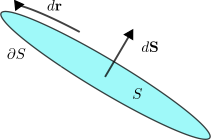
in Figure 21.
The right-hand rule of orientation in Stokes’
theorem.
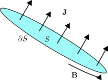
Ampère’s law relating the current flux to a line integral of
magnetic field.Applying Stokes’ theorem to Ampère’s law.
Integrating both sides of \(\eqref{eq:max_bstatic_curl}\) over \(S\) yields, \[\begin{aligned}
\int_S\,\left(\nabla\times\mathbf{B}\right)\cdot d\mathbf{S} &=
\mu_0\,\int_S\,\mathbf{J}\cdot d\mathbf{S}=\mu_0\,I_S\,,
\end{aligned}\] where we used that the surface integral of the
current density gives the electric current flow3
through \(S\). Applying Stokes’ theorem
to the left-hand side gives the integral form of Ampère’s
law,
Similarly to Gauss’ law in electrostatics, this integral form will
help us build intuition for the general behaviour of magnetic
fields.
Magnetic fields are generated by currents according to the same
right-hand rule that appears in Stokes’ theorem. To see this, suppose
that the electric current density \(\mathbf{J}\) points in the same direction
across the whole surface \(S\). Without
loss of generality, choose the orientation \(d\mathbf{S}\) to point along \(\mathbf{J}\), in the sense that the inner
product of the unit normal \(\hat{\mathbf{n}}\) with \(\mathbf{J}\) is everywhere positive. This
makes the current flux \(I_S\)
positive, so the line integral of the resulting \(\mathbf{B}\) must also be positive.
Therefore \(\mathbf{B}\) has to
circulate in the direction of \(d\mathbf{r}\) determined by the right-hand
rule. The resulting rule is illustrated in Figure 23.
The line integral of the magnetic field over a curve \(C\) depends only on the flux of the current
density it encloses. This suggests that we are free to deform \(C\) as we wish, as long as the current
passing through it remains unchanged.
As in the case of Gauss’ law, Ampère’s law will allow us to determine
\(\mathbf{B}\) completely in simple
geometries. Once again, we stress that the divergence free condition
\(\eqref{eq:max_bstatic_div}\) needs to
be taken into account simultaneously.
5.2 The
Infinitely Long Wire
As a first magnetostatic example, consider an infinitely long,
straight wire carrying a steady current \(I\). The system is invariant under
rotations about the wire and under translations along it. It is
therefore natural to use cylindrical coordinates \((r,\phi,z)\) and place the wire on the
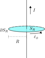
\(z\)-axis, as shown in Figure 24.
Geometry for an infinitely long straight wire.
The symmetry immediately constrains the form of \(\mathbf{B}\). Translation invariance along
the wire implies no \(z\)-dependence,
while rotational invariance implies no \(\phi\)-dependence. Moreover, the field
lines must circle the wire, so the direction of \(\mathbf{B}\) is azimuthal. We therefore
make the ansatz, \[\begin{align}
\label{eq:infinite_wire_ansatz}
\mathbf{B}(\mathbf{r})=B(r)\,\hat{\mathbf{e}}_\phi\,.
\end{align}\] It is straightforward to check that \(\eqref{eq:infinite_wire_ansatz}\) satisfies
the divergence-free condition \(\eqref{eq:max_bstatic_div}\).
To determine the function \(B(r)\),
apply Ampère’s law \(\eqref{eq:ampere_law}\) to a disc \(S_R\) of radius \(R\) orthogonal to the wire and centred on
the \(z\)-axis. The current piercing
this surface is simply \(I_{S_R}=I\).
On the boundary circle \(\partial S_R\)
we have \(r=R\) and, \[\begin{aligned}
d\mathbf{r}=R\,\hat{\mathbf{e}}_\phi\,d\phi\,,
\end{aligned}\] so the line integral becomes, \[\begin{aligned}
\int_{\partial S_R}\mathbf{B}(\mathbf{r})\cdot d\mathbf{r}
&=\int_{0}^{2\pi}
B(R)\,\hat{\mathbf{e}}_\phi\cdot\left(R\,\hat{\mathbf{e}}_\phi\,d\phi\right)
=2\pi R\,B(R)\,.
\end{aligned}\] Ampère’s law then gives \(2\pi R\,B(R)=\mu_0 I\), and hence, \[\begin{aligned}
\mathbf{B}(\mathbf{r})=\frac{\mu_0\,I}{2\pi r}\,\hat{\mathbf{e}}_\phi\,.
\end{aligned}\]
This result relied heavily on symmetry. Later, after introducing the
vector potential and the Biot–Savart law, we will return to this example
as a useful check of the general formalism.
5.3
Surface Currents
We begin with the simplest magnetostatic example involving a surface
current. An infinite plane \(S\)
carrying a constant surface current density \(\mathbf{K}\). The most obvious symmetries
are translations parallel to the surface. In addition, there is a less
obvious discrete symmetry, a \(\ang{180}\) rotation about an axis lying in
\(S\) and parallel to \(\mathbf{K}\).
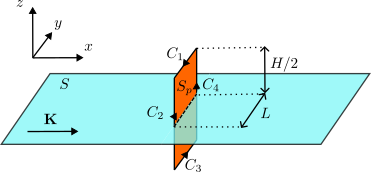
The infinite plane with constant surface current
density.
We work in Cartesian coordinates, taking \(S\) to be the plane \(z=0\) and choosing the surface current
density to be \(\mathbf{K}=K\,\hat{\mathbf{e}}_x\), as
shown in Figure 25.
From the example of the infinite wire in the previous section, we expect
\(\mathbf{B}\) to be orthogonal to
\(\mathbf{K}\), so it should lie in the
span of \(\hat{\mathbf{e}}_y\) and
\(\hat{\mathbf{e}}_z\). Translation
invariance in the \(x\) and \(y\) directions implies that \(\mathbf{B}\) can depend only on \(z\), so we make the ansatz, \[\begin{align}
\label{eq:infinite_plane_B_ansatz}
\mathbf{B}(\mathbf{x}) =
B_y(z)\,\hat{\mathbf{e}}_y+B_z(z)\,\hat{\mathbf{e}}_z\,.
\end{align}\] Under the \(\ang{180}\) rotation mentioned above, \(\hat{\mathbf{e}}_y\mapsto
-\hat{\mathbf{e}}_y\) and \(\hat{\mathbf{e}}_z\mapsto
-\hat{\mathbf{e}}_z\), while \(z\mapsto
-z\). Invariance of the magnetic field therefore imposes, \[\begin{align}
\label{eq:infinite_plane_B_sym}
B_y(-z)=-B_y(z), \qquad B_z(-z)=-B_z(z)\,.
\end{align}\]
Imposing the divergence-free condition \(\eqref{eq:max_bstatic_div}\) on \(\eqref{eq:infinite_plane_B_ansatz}\) gives,
\[\begin{aligned}
\partial_z B_z(z)=0\,,
\end{aligned}\] so \(B_z\) must
be a constant. The only function that is both constant and odd is the
trivial one, hence, \[\begin{aligned}
B_z(z)=0\,.
\end{aligned}\] The magnetic field therefore reduces to, \[\begin{align}
\label{eq:infinite_plane_B_ansatz_2}
\mathbf{B}(\mathbf{x}) = B(z)\,\hat{\mathbf{e}}_y\,,
\end{align}\] with \(B(-z)=-B(z)\).
We now use the integral form of Ampère’s law \(\eqref{eq:ampere_law}\) to determine \(B(z)\). Consider a rectangular surface
\(S_p\) of height \(H\) and length \(L\), with sides parallel to the \(z\)- and \(y\)-axes, intersecting the plane \(S\) as shown in Figure 25. To apply Ampère’s law we
need the current flux through \(S_p\).
As discussed in Section 2.2,
we use \(\eqref{eq:curr_flux_surf}\)
and integrate \(\mathbf{K}\) over the
intersection \(S_p\cap S\), obtaining,
\[I_{S_p}=I_{S_p\cap S}=K\,L\,,\]
since \(\mathbf{K}\) is orthogonal to
\(S_p\cap S\).
Next, compute the line integral around the boundary \(\partial S_p\). Decompose \(\partial S_p=C_1\cup C_2\cup C_3\cup C_4\)
with the orientations shown in Figure 25,
and write, \[\begin{aligned}
\int_{\partial S_p}\mathbf{B}\cdot d\mathbf{r}
=\int_{C_1}\mathbf{B}\cdot d\mathbf{r}_1 + \int_{C_2}\mathbf{B}\cdot
d\mathbf{r}_2 +\int_{C_3}\mathbf{B}\cdot d\mathbf{r}_3 +
\int_{C_4}\mathbf{B}\cdot d\mathbf{r}_4\,.
\end{aligned}\] Along these segments we have, \[\begin{aligned}
d\mathbf{r}_1 =- \hat{\mathbf{e}}_y\,dy\,,\quad
d\mathbf{r}_2 =- \hat{\mathbf{e}}_z\,dz\,,\quad
d\mathbf{r}_3 = \hat{\mathbf{e}}_y\,dy\,,\quad
d\mathbf{r}_4 =\hat{\mathbf{e}}_z\,dz\,.
\end{aligned}\] The integrals along \(C_2\) and \(C_4\) vanish because \(d\mathbf{r}\) is orthogonal to \(\mathbf{B}\propto \hat{\mathbf{e}}_y\). For
the remaining two segments, \[\begin{aligned}
\int_{C_1}\mathbf{B}\cdot d\mathbf{r}_1&=
-B(H/2)\int_{C_1}dy=-B(H/2)\,L\,,\notag\\
\int_{C_3}\mathbf{B}\cdot d\mathbf{r}_3&= B(-H/2)\int_{C_3}dy=
B(-H/2)\,L\,.
\end{aligned}\] Ampère’s law \(\eqref{eq:ampere_law}\) then gives, \[\begin{aligned}
&-B(H/2)\,L+B(-H/2)\,L=\mu_0\,K\,L\Rightarrow \notag\\
&B(H/2)=-\frac{\mu_0\,K}{2}\,,
\end{aligned}\] where we used that \(B\) is odd. Since \(H\) is arbitrary, this determines \(B(z)\) for all \(z\neq 0\), and we find, \[\begin{aligned}
\mathbf{B}(\mathbf{x})=\begin{cases}
-\frac{\mu_0\,K}{2}\,\hat{\mathbf{e}}_y,& z>0\\
\frac{\mu_0\,K}{2}\,\hat{\mathbf{e}}_y,& z<0\\
\end{cases}\,,
\end{aligned}\] showing that the field is constant on each side
of the surface current.
The rest of this subsection is non-examinable.
As in the electrostatic example of an infinite uniformly charged
plane, the field is discontinuous across the surface. Denoting by \(\mathbf{B}_\pm\) the limits as \(z\to 0^\pm\), the discontinuity is in the
component parallel to the plane, \[\begin{aligned}
\mathbf{B}_+-\mathbf{B}_- = -\mu_0\,K\,\hat{\mathbf{e}}_y\,,
\end{aligned}\] which can be written in a coordinate-free form
as,
where \(\hat{\mathbf{n}}=\hat{\mathbf{e}}_z\) is
the unit normal to \(S\). In contrast
to the electric field, the component of \(\mathbf{B}\) normal to the surface is
continuous,
These discontinuity conditions hold for a general surface \(S\) carrying a surface current density
\(\mathbf{K}\). The derivation
parallels that of Section 4.5, but in
magnetostatics the continuity properties are reversed, \(\mathbf{B}\) has zero divergence but a
sourced curl.
5.4 The
Vector Potential
In Section 4.6 we discussed the
consequences of the curl-free nature of the electrostatic field which
allows us to introduce a scalar potential. In magnetostatics the
corresponding structural equation is instead the absence of magnetic
charge, and this leads naturally to the introduction of the vector
potential. The following remarks rely only on \(\eqref{eq:max_3}\) and therefore remain
true even in time-dependent electromagnetism.
By integrating both sides of equation \(\eqref{eq:max_bstatic_div}\) over a volume
region \(V\) and using Gauss’ theorem,
we conclude that,
Magnetic flux through surfaces with a common
boundary.
A useful consequence of \(\eqref{eq:magnetic_flux_through_closed_surface}\)
is that the magnetic flux through an open surface depends only on its
boundary loop. Consider two open surfaces \(S_1\) and \(S_2\) with the same boundary curve \(C\), \(\partial
S_1=C=\partial S_2\), but with opposite induced orientations on
\(C\) (as in Figure 26). The union \(S_1\cup S_2\) then forms a closed surface,
so, \[\begin{aligned}
\oint_{S_1\cup S_2}\mathbf{B}\cdot d\mathbf{S}=0\,.
\end{aligned}\] Decomposing the closed-surface integral gives,
\[\begin{aligned}
&\int_{S_1}\mathbf{B}\cdot d\mathbf{S}_1+\int_{S_2}\mathbf{B}\cdot
d\mathbf{S}_2=0\Rightarrow\notag\\
&\int_{S_1}\mathbf{B}\cdot d\mathbf{S}_1=-\int_{S_2}\mathbf{B}\cdot
d\mathbf{S}_2\,.
\end{aligned}\] In other words, once the boundary orientation is
fixed, the flux through any spanning surface is the same. This motivates
defining the magnetic flux through the loop \(C\) as the flux through any surface
with boundary \(C\).
The condition \(\eqref{eq:max_3}\)
also suggests a stronger statement. Locally, a divergence-free vector
field can be written as the curl of another vector field. This motivates
the following definition,
where \(\mathbf{A}\) is called the
vector potential. By construction, \(\eqref{eq:vector_potential}\) automatically
satisfies \(\eqref{eq:max_3}\) because
of property \(\eqref{eq:prop_1}\).
The vector potential is not uniquely determined by \(\mathbf{B}\). Indeed, if \(\chi(\mathbf{x})\) is any smooth scalar
function, then the gauge transformation,
leaves the magnetic field unchanged, \[\begin{aligned}
\nabla\times\mathbf{A}^\prime=\nabla\times\mathbf{A}+\nabla\times(\nabla\chi)=\nabla\times\mathbf{A}=\mathbf{B}\,,
\end{aligned}\] using \(\eqref{eq:prop_2}\). This is the gauge
symmetry of the vector potential.
Substituting \(\eqref{eq:vector_potential}\) into Ampère’s
law \(\eqref{eq:max_bstatic_curl}\)
yields an equation determining \(\mathbf{A}\) in terms of the current
density,
To actually solve for \(\mathbf{A}\), we will need to deal with the
fact that \(\mathbf{A}\) is not unique
due to remark [rem:vector_potential_gauge_transformation].
This non-uniqueness is the magnetic analogue of the freedom to shift the
scalar potential by a constant in electrostatics, but now it is a
local freedom. We will therefore need to fix this freedom by
imposing an additional gauge fixing condition or gauge
choice condition,
where \(\mathcal{G}\) is a scalar
function of the vector potential \(\mathbf{A}\). We will see a specific gauge
choice in the next subsection.
A classical particle of mass \(m\)
and charge \(q\) experiences the
Lorentz force \(m\ddot{\mathbf{x}}=q\,\dot{\mathbf{x}}\times\mathbf{B}\).
Using \(\mathbf{B}=\nabla\times\mathbf{A}\), one
can show that these equations follow from a variational principle with
Lagrangian, \[\begin{align}
\label{eq:magnetic_field_lagrangian}
L=\frac{1}{2}m\,\dot{\mathbf{x}}^2+q\,\dot{\mathbf{x}}\cdot
\mathbf{A}(\mathbf{x}(t))\,.
\end{align}\] Under the gauge transformation \(\mathbf{A}\mapsto\mathbf{A}+\nabla\chi\),
the Lagrangian changes by a total time derivative, \(L\mapsto
L+q\,\frac{d}{dt}\chi(\mathbf{x}(t))\), so the equations of
motion are unchanged. Gauge invariance is therefore built directly into
the variational description.
Suppose that the open surface \(S\)
has \(C=\partial S\) as its closed
boundary. Using Stokes’ theorem together with \(\eqref{eq:vector_potential}\), we can
express the flux of \(\mathbf{B}\)
through \(S\) as a line integral over
\(\mathbf{A}\), \[\begin{align}
\label{eq:magnetic_flux_as_line_integral}
\int_S \mathbf{B}\cdot d\mathbf{S}=\oint_C \mathbf{A}\cdot
d\mathbf{r}\,.
\end{align}\] This is often the most convenient way to compute
magnetic fluxes in practice.
Given vanishing boundary conditions at infinity for the magnetic
field, the vector potential is additive. If \(\mathbf{B}=\mathbf{B}_1+\mathbf{B}_2\) with
corresponding potentials \(\mathbf{A}_1\) and \(\mathbf{A}_2\), then \(\mathbf{A}=\mathbf{A}_1+\mathbf{A}_2\) is a
potential for \(\mathbf{B}\) (up to a
gauge transformation).
All of the above remarks, except for equation \(\eqref{eq:vector_potential_equation}\),
also hold in the time-dependent case, provided only that \(\nabla\cdot\mathbf{B}=0\). This is always
true for the magnetic field. In contrast, the equation determining \(\mathbf{A}\) from the sources changes once
time dependence is included.
5.5
Biot–Savart Law
In this section we derive an explicit expression for the magnetic
field produced by a general static current density \(\mathbf{J}(\mathbf{x})\). We do this by
solving the vector potential equation \(\eqref{eq:vector_potential_equation}\) for
\(\mathbf{A}\), and then computing
\(\mathbf{B}\) via \(\eqref{eq:vector_potential}\). Throughout
we assume that the current density decays sufficiently fast at infinity,
in particular faster than \(1/|\mathbf{x}|^2\) as \(|\mathbf{x}|\to\infty\).
As we discussed in the previous section, solving \(\eqref{eq:vector_potential_equation}\)
requires an appropriate choice of gauge. A convenient choice is the
Coulomb gauge, \[\begin{align}
\label{eq:coulomb_gauge}
\mathcal{G}(\mathbf{A})= \nabla\cdot\mathbf{A}=0\,.
\end{align}\] To see why this is always achievable, suppose \(\tilde{\mathbf{A}}\) is any solution of
\(\eqref{eq:vector_potential_equation}\) and
define \(\psi=\nabla\cdot\tilde{\mathbf{A}}\). By
Remark [rem:vector_potential_gauge_transformation]
we may perform a gauge transformation, \[\begin{aligned}
\mathbf{A}=\tilde{\mathbf{A}}+\nabla\chi\,,
\end{aligned}\] without changing the magnetic field. We obtain,
\[\begin{aligned}
\nabla\cdot\mathbf{A}=\nabla\cdot\tilde{\mathbf{A}}+\nabla^2\chi=\psi+\nabla^2\chi\,,
\end{aligned}\] so imposing the Coulomb gauge amounts to solving,
\[\begin{aligned}
\nabla^2\chi=-\psi\,,
\end{aligned}\] with boundary conditions such that \(\chi\) vanishes at infinity. This is
precisely the same Poisson problem that appears in electrostatics (see
4.7), after the
identifications \(\chi\leftrightarrow
\varphi\) and \(\psi\leftrightarrow
\rho/\varepsilon_0\).
In Coulomb gauge, the vector potential equation \(\eqref{eq:vector_potential_equation}\)
simplifies by imposing \(\eqref{eq:coulomb_gauge}\), and we obtain,
\[\begin{aligned}
\nabla^2\mathbf{A}=-\mu_0\,\mathbf{J}\,.
\end{aligned}\] In Cartesian coordinates this is the
component-wise Poisson equation, \[\begin{align}
\label{eq:vector_potential_equation_coulomb_gauge}
\nabla^2 A_i=-\mu_0\,J_i\,,
\end{align}\] which is a multi-component generalisation of \(\eqref{eq:electrostatic_spontential_eq}\).
Therefore, by the same Green’s-function method used in \(\eqref{eq:scalar_potential_general_sol}\),
the solution for each component is, \[\begin{aligned}
A_i(\mathbf{x})=\frac{\mu_0}{4\pi}\int_{\mathbb{R}^3}\frac{J_i(\mathbf{x}^\prime)}{|\mathbf{x}-\mathbf{x}^\prime|}\,d^3\mathbf{x}^\prime\,.
\end{aligned}\] or, equivalently, in vector notation,
where the components of \(\mathbf{A}\) pair with the components of
\(\mathbf{J}\) in the integrand when
written in Cartesian coordinates.
This might be the first time you encounter an integral producing a
vector. A useful property is that given a function \(f(\mathbf{x})\) and a constant vector \(\mathbf{v}\), you can write, \[\int_V
f(\mathbf{x})\,\mathbf{v}\,d^3\mathbf{x}=\left(\int_V f(\mathbf{x})\,
d^3\mathbf{x}\right)\,\mathbf{v}\,.\] For example, if a vector
field \(\mathbf{C}(\mathbf{x})\) is
decomposed in a Cartesian basis \(\mathbf{C}(\mathbf{x})=C_x(\mathbf{x})\,\hat{\mathbf{e}}_x+C_y(\mathbf{x})\,\hat{\mathbf{e}}_y+C_z(\mathbf{x})\,\hat{\mathbf{e}}_z\),
then, \[\int_V
\mathbf{C}(\mathbf{x})\,d^3\mathbf{x}=\left(\int_V
C_x(\mathbf{x})\,d^3\mathbf{x} \right)\,\hat{\mathbf{e}}_x+\left(\int_V
C_y(\mathbf{x})\,d^3\mathbf{x} \right)\,\hat{\mathbf{e}}_y+\left(\int_V
C_z(\mathbf{x})\,d^3\mathbf{x} \right)\,\hat{\mathbf{e}}_z\,.\]
However, decomposing in e.g. cylindrical coordinates basis \(\mathbf{C}(\mathbf{x})=C_r(\mathbf{x})\,\hat{\mathbf{e}}_r+C_\phi(\mathbf{x})\,\hat{\mathbf{e}}_\phi+C_z(\mathbf{x})\,\hat{\mathbf{e}}_z\),
allows us to write only, \[\int_V
\mathbf{C}(\mathbf{x})\,d^3\mathbf{x}=\int_V
C_r(\mathbf{x})\,\hat{\mathbf{e}}_r\,d^3\mathbf{x} +\int_V
C_\phi(\mathbf{x})\,\hat{\mathbf{e}}_\phi\,d^3\mathbf{x} +\left(\int_V
C_z(\mathbf{x})\,d^3\mathbf{x} \right)\,\hat{\mathbf{e}}_z\,,\]
since the only constant basis vector is \(\hat{\mathbf{e}}_z\).
As a sanity check, we verify that \(\eqref{eq:vector_potential_general_sol}\)
indeed satisfies Coulomb gauge provided \(\mathbf{J}\) is divergence free, as it must
be in a steady configuration. Taking the divergence with respect to
\(\mathbf{x}\) gives, \[\begin{aligned}
\nabla_{\mathbf{x}}\cdot \mathbf{A}(\mathbf{x})
&=\frac{\mu_0}{4\pi}\,\nabla_{\mathbf{x}}\cdot\left(\int_{\mathbb{R}^3}\frac{\mathbf{J}(\mathbf{x}^\prime)}{|\mathbf{x}-\mathbf{x}^\prime|}\,d^3\mathbf{x}^\prime\right)\notag\\
&=\frac{\mu_0}{4\pi}\,\int_{\mathbb{R}^3}\mathbf{J}(\mathbf{x}^\prime)\cdot\nabla_{\mathbf{x}}\!\left(\frac{1}{|\mathbf{x}-\mathbf{x}^\prime|}\right)\,d^3\mathbf{x}^\prime\notag\\
&=-\frac{\mu_0}{4\pi}\,\int_{\mathbb{R}^3}\mathbf{J}(\mathbf{x}^\prime)\cdot\nabla_{\mathbf{x}^\prime}\!\left(\frac{1}{|\mathbf{x}-\mathbf{x}^\prime|}\right)\,d^3\mathbf{x}^\prime\notag\\
&=\frac{\mu_0}{4\pi}\,\int_{\mathbb{R}^3}\left(\nabla_{\mathbf{x}^\prime}\cdot\mathbf{J}(\mathbf{x}^\prime)\right)\,\frac{1}{|\mathbf{x}-\mathbf{x}^\prime|}\,d^3\mathbf{x}^\prime\,,
\end{aligned}\] where in the last step we integrated by parts and
used the assumed fall-off at infinity to discard the boundary term. For
a steady current, \(\nabla\cdot\mathbf{J}=0\), so the final
expression vanishes and \(\eqref{eq:coulomb_gauge}\) is
satisfied.
We now compute the magnetic field by taking the curl of \(\eqref{eq:vector_potential_general_sol}\).
Since \(\mathbf{J}(\mathbf{x}^\prime)\)
depends only on the integration variable, the \(\mathbf{x}\)-curl acts only on the
Green’s-function kernel, \[\begin{aligned}
\mathbf{B}(\mathbf{x})=\nabla\times_{\mathbf{x}}\mathbf{A}(\mathbf{x})
&=\frac{\mu_0}{4\pi}\int_{\mathbb{R}^3}\nabla{\mathbf{x}}\times\!\left(\frac{\mathbf{J}(\mathbf{x}^\prime)}{|\mathbf{x}-\mathbf{x}^\prime|}\right)\,d^3\mathbf{x}^\prime\notag\\
&=\frac{\mu_0}{4\pi}\int_{\mathbb{R}^3}\nabla_{\mathbf{x}}\!\left(\frac{1}{|\mathbf{x}-\mathbf{x}^\prime|}\right)\times
\mathbf{J}(\mathbf{x}^\prime)\,d^3\mathbf{x}^\prime\notag\\
&=\frac{\mu_0}{4\pi}\int_{\mathbb{R}^3}\frac{\mathbf{J}(\mathbf{x}^\prime)\times\left(\mathbf{x}-\mathbf{x}^\prime\right)}{|\mathbf{x}-\mathbf{x}^\prime|^3}\,d^3\mathbf{x}^\prime\,.
\end{aligned}\] This is the Biot–Savart law for a
general current density,
A common special case is a current confined to a thin wire along a
curve \(C\), parametrised by \(\mathbf{r}(s)\) and carrying current \(I(s)\). In that case the volume current
density can be written as \(\eqref{eq:curr_density_curve}\).
Substituting it into \(\eqref{eq:biot_savart}\) and performing the
\(\mathbf{x}^\prime\) integral using
the Dirac delta gives,
We now recover the magnetic field of an infinitely long straight wire,
previously obtained in Section 5.2, as a check of \(\eqref{eq:biot_savart_curve}\). Work in
cylindrical coordinates and parametrise the wire by, \[\begin{aligned}
\mathbf{r}(s)=s\,\hat{\mathbf{e}}_z\,,\qquad I(s)=I\,,
\end{aligned}\] while the observation point is \(\mathbf{x}=r\,\hat{\mathbf{e}}_r+z\,\hat{\mathbf{e}}_z\).
Then, \[\begin{aligned}
\dot{\mathbf{r}}(s)\times\left(\mathbf{x}-\mathbf{r}(s)\right)
&=\hat{\mathbf{e}}_z\times\left(r\,\hat{\mathbf{e}}_r+(z-s)\,\hat{\mathbf{e}}_z\right)
=r\,\hat{\mathbf{e}}_z\times\hat{\mathbf{e}}_r
=r\,\hat{\mathbf{e}}_\phi\,,\notag\\
|\mathbf{x}-\mathbf{r}(s)|^2&=(z-s)^2+r^2\,.
\end{aligned}\] Substituting into \(\eqref{eq:biot_savart_curve}\) yields,
\[\begin{aligned}
\mathbf{B}(\mathbf{x})
&=\frac{\mu_0\,I}{4\pi}\left(\int_{-\infty}^{+\infty}\frac{r}{\left((z-s)^2+r^2\right)^{3/2}}\,ds\right)\hat{\mathbf{e}}_\phi\notag\\
&\overset{s=z+r\tan\theta}{=}\frac{\mu_0\,I}{4\pi\,r}\left(\int_{-\pi/2}^{+\pi/2}\cos\theta\,d\theta\right)\hat{\mathbf{e}}_\phi\notag\\
&=\frac{\mu_0\,I}{2\pi\,r}\,\hat{\mathbf{e}}_\phi\,,
\end{aligned}\] in agreement with our previous result.
5.6 The
Multipole Expansion
As in the electrostatic case discussed in Section 4.8, we can use the general
solution for the vector potential \(\eqref{eq:vector_potential_general_sol}\)
to study the magnetic field far away from its sources. We assume that
the current density \(\mathbf{J}(\mathbf{x}^\prime)\) is
localised inside some bounded region \(V\), and we evaluate the vector potential
at observation points \(\mathbf{x}\)
satisfying \(|\mathbf{x}|\gg
|\mathbf{x}^\prime|\) for all \(\mathbf{x}^\prime\in V\). Substituting the
large-distance expansion \(\eqref{eq:large_distance_exp}\) into \(\eqref{eq:vector_potential_general_sol}\)
gives, \[\begin{aligned}
\mathbf{A}(\mathbf{x})=\frac{\mu_0}{4\pi}\left(
\frac{1}{|\mathbf{x}|}\int_V\mathbf{J}(\mathbf{x}^\prime)\,d^3\mathbf{x}^\prime+\frac{1}{|\mathbf{x}|^3}\,\int_V\mathbf{J}(\mathbf{x}^\prime)\,\left(\mathbf{x}\cdot
\mathbf{x}^\prime \right)\,d^3\mathbf{x}^\prime+\cdots\right)\,.
\end{aligned}\] For later use it is convenient to write this
expansion in components, \[\begin{align}
\label{eq:vector_potential_expansion}
A_i(\mathbf{x})=\frac{\mu_0}{4\pi}\left( \frac{1}{|\mathbf{x}|}\int_V
J_i(\mathbf{x}^\prime)\,d^3\mathbf{x}^\prime+\frac{1}{|\mathbf{x}|^3}\,\int_V
J_i(\mathbf{x}^\prime)\,x_j\,x_j^\prime\,d^3\mathbf{x}^\prime+\cdots\right)\,.
\end{align}\]
At first sight, the leading term in \(\eqref{eq:vector_potential_expansion}\)
might look like a “magnetic monopole” contribution, in tension with
Remark [rem:magnetic_monopoles]. In
fact, for a steady current it vanishes. To see this, use equation \(\eqref{eq:J_div}\) and note that, \[\begin{aligned}
\partial_j^\prime\left(J_j(\mathbf{x}^\prime)\,x_i^\prime
\right)&=x_i^\prime \,\partial_j^\prime
J_j(\mathbf{x}^\prime)+J_j(\mathbf{x}^\prime)\,\partial_j^\prime
x_i^\prime=x_i^\prime \,\partial_j^\prime
J_j(\mathbf{x}^\prime)+J_j(\mathbf{x}^\prime)\,\delta_{ji}\notag\\
&=x_i^\prime \,\partial_j^\prime
J_j(\mathbf{x}^\prime)+J_i(\mathbf{x}^\prime)\notag\\
&=J_i(\mathbf{x}^\prime)\,,
\end{aligned}\] where \(\partial^\prime\) denotes derivatives with
respect to the primed coordinates. Integrating over \(V\) and applying Gauss’ theorem yields,
\[\begin{align}
\label{eq:current_integral}
\int_V J_i(\mathbf{x}^\prime)\,d^3\mathbf{x}^\prime=\int_V
\partial_j^\prime\left(J_j(\mathbf{x}^\prime)\,x_i^\prime
\right)\,d^3\mathbf{x}^\prime
=\oint_{\partial V}\left(\mathbf{J}(\mathbf{x}^\prime)\cdot
\hat{\mathbf{n}}\right)\,x_i^\prime\,dS\,.
\end{align}\] Since the current is localised, we may choose \(V\) so that \(\mathbf{J}=0\) on \(\partial V\), and the surface term
vanishes. Therefore the monopole-like contribution in \(\eqref{eq:vector_potential_expansion}\) is
absent.
The leading non-zero term is therefore the second term in \(\eqref{eq:vector_potential_expansion}\). To
simplify it, observe that, \[\begin{aligned}
\partial_j^\prime\left(J_j(\mathbf{x}^\prime)\,x_i^\prime\,x_k^\prime
\right)=x_i^\prime\,J_k(\mathbf{x}^\prime)+x_k^\prime\,J_i(\mathbf{x}^\prime)\,,
\end{aligned}\] which again follows from \(\eqref{eq:J_div}\). Integrating over \(V\) and using the same boundary conditions
gives, \[\begin{align}
\label{eq:current_integral_trick}
\int_V x_i^\prime\,J_k(\mathbf{x}^\prime)\,d^3\mathbf{x}^\prime =-
\int_V x_k^\prime\,J_i(\mathbf{x}^\prime)\,d^3\mathbf{x}^\prime\,.
\end{align}\] We can therefore exchange the indices at the cost
of a minus sign. Using this identity, we rewrite, \[\begin{aligned}
\int_V
J_i(\mathbf{x}^\prime)\,x_j\,x_j^\prime\,d^3\mathbf{x}^\prime&=x_j\,\int_V
J_i(\mathbf{x}^\prime)\,x_j^\prime\,d^3\mathbf{x}^\prime\notag\\
&=\frac{1}{2}x_j\,\int_V
\left(J_i(\mathbf{x}^\prime)\,x_j^\prime+J_i(\mathbf{x}^\prime)\,x_j^\prime\right)\,d^3\mathbf{x}^\prime\notag\\
&=\frac{1}{2}x_j\,\int_V
\left(J_i(\mathbf{x}^\prime)\,x_j^\prime-J_j(\mathbf{x}^\prime)\,x_i^\prime\right)\,d^3\mathbf{x}^\prime\notag\\
&=\frac{1}{2}\int_V \left(\left(\mathbf{x}\cdot \mathbf{x}^\prime
\right)\,J_i(\mathbf{x}^\prime)-\left(\mathbf{J}(\mathbf{x}^\prime)\cdot
\mathbf{x}\right)\,x_i^\prime\right)\,d^3\mathbf{x}^\prime\notag\\
&=\frac{1}{2}\,\int_V\left[\mathbf{x}\times\left(\mathbf{J}(\mathbf{x}^\prime)
\times \mathbf{x}^\prime\right) \right]_i\,d^3\mathbf{x}^\prime\notag\\
&=(\mathbf{m}\times \mathbf{x})_i\,,
\end{aligned}\] where we introduced the magnetic dipole
moment of the current distribution,
The corresponding magnetic field follows from \(\eqref{eq:vector_potential}\). Using the
vector identity \(\eqref{eq:prop_5}\),
we obtain, \[\begin{aligned}
\mathbf{B}(\mathbf{x})=\nabla\times\mathbf{A}(\mathbf{x})=\frac{\mu_0}{4\pi}\left[\mathbf{m}\,
\nabla\cdot\left(\frac{\mathbf{x}}{|\mathbf{x}|^3}\right)-\left(
\mathbf{m}\cdot\nabla\right)\left(\frac{\mathbf{x}}{|\mathbf{x}|^3}\right)
\right] + \cdots\,.
\end{aligned}\] For \(\mathbf{x}\neq
0\) we have \(\nabla\cdot(\mathbf{x}/|\mathbf{x}|^3)=0\),
so the first term vanishes, and the second term gives the familiar
dipole field,
which has the same functional form as the electric dipole
contribution in \(\eqref{eq:electric_field_asymptotic_behaviour}\).
We have derived \(\eqref{eq:magnetic_field_dipole}\) by
analysing the long-distance behaviour of classical current
distributions. However, magnetic dipole moments also arise more
fundamentally. In quantum mechanics, particles with spin typically carry
an intrinsic magnetic dipole moment.
We now compute \(\mathbf{m}\) for a
current confined to a thin wire along a closed curve \(C\). Using the curve current density \(\eqref{eq:curr_density_curve}\) in \(\eqref{eq:magnetic_dipole_moment}\)
gives,
We consider a circular loop of radius \(R\) carrying a constant current \(I\). Place its centre at the origin and
take it to lie in the \(z=0\) plane. If
the current runs counterclockwise in the \(x\)–\(y\)
plane, a convenient parametrisation is, \[\begin{aligned}
\mathbf{r}(s)=R\,\left(\cos\left(s\right)\,\hat{\mathbf{e}}_x+\sin\left(s
\right)\,\hat{\mathbf{e}}_y\right)\,,
\end{aligned}\] with \(s\in\left[0,2\pi\right)\). Then, \[\begin{aligned}
\mathbf{r}(s)\times \dot{\mathbf{r}}(s)=R^2\,\hat{\mathbf{e}}_z\,,
\end{aligned}\] and \(\eqref{eq:magnetic_dipole_moment_loop}\)
yields, \[\begin{aligned}
\mathbf{m}=\frac{R^2I}{2}\,\int_0^{2\pi}ds\,\hat{\mathbf{e}}_z=I\,S\,\hat{\mathbf{e}}_z\,,
\end{aligned}\] where \(S=\pi
R^2\) is the area enclosed by the loop.
This example shows that the dipole moment is determined by a simple
geometric property of the loop. More generally, for any planar closed
curve \(C\) carrying a constant current
\(I\), the magnetic dipole moment can
be written as,
where \(S_C\) is the area enclosed
by \(C\) and \(\hat{\mathbf{n}}\) is the unit normal to
the plane, determined by the right-hand rule.
5.7
Force and Potential for a Dipole
In this section we study how a spatially localised current
distribution \(\mathbf{J}\) interacts
with an external magnetic field \(\mathbf{B}\). Concretely, we analyse the
Lorentz force, \[\begin{align}
\label{eq:force_dipole}
\mathbf{F}=\int_V \mathbf{J}(\mathbf{x})\times
\mathbf{B}(\mathbf{x})\,d^3\mathbf{x}
\end{align}\] exerted on the current distribution. We assume that
we are sufficiently far from the sources of \(\mathbf{B}\) so that, throughout the region
\(V\) occupied by the current, \[\begin{align}
\label{eq:curl_free_B}
\nabla\times\mathbf{B}(\mathbf{x})=0\,,
\end{align}\] for any \(\mathbf{x}\in
V\).
To make progress with the integral in \(\eqref{eq:force_dipole}\), we Taylor expand
the magnetic field about a reference point \(\mathbf{x}_0\) associated with the
distribution e.g. its centre of mass. For notational simplicity we
choose coordinates so that \(\mathbf{x}\) denotes the displacement from
\(\mathbf{x}_0\). The expansion reads,
\[\begin{aligned}
\mathbf{B}(\mathbf{x})=\mathbf{B}(\mathbf{x}_0)+\left(\left(\mathbf{x}-\mathbf{x}_0
\right)\cdot \nabla\right)\mathbf{B}(\mathbf{x}_0)+\cdots\,.
\end{aligned}\] Substituting this expansion into \(\eqref{eq:force_dipole}\), and using \(\eqref{eq:current_integral}\) to drop the
leading term proportional to \(\mathbf{B}(\mathbf{x}_0)\), we obtain,
\[\begin{aligned}
\mathbf{F}=\int_V \mathbf{J}(\mathbf{x})\times
\left(\left(\mathbf{x}\cdot \nabla
\right)\mathbf{B}(\mathbf{x}_0)\right)\,d^3\mathbf{x}\,.
\end{aligned}\] Writing this expression in component notation
gives, \[\begin{aligned}
F_i&=\varepsilon_{ijk}\,\int_V J_j(\mathbf{x})\,x_l \,
\partial_{x_{0l}}B_k(\mathbf{x}_0)\,d^3\mathbf{x}\overset{\eqref{eq:curl_free_B}}{=}
\varepsilon_{ijk}\,\int_V J_j(\mathbf{x})\,x_l \,
\partial_{x_{0k}}B_l(\mathbf{x}_0)\,d^3\mathbf{x}\notag\\
&=\varepsilon_{ijk}\,\partial_{x_{0k}}\int_V J_j(\mathbf{x})\,x_l \,
B_l(\mathbf{x}_0)\,d^3\mathbf{x}\overset{\eqref{eq:current_integral_trick}}{=}
\frac{1}{2}\varepsilon_{ijk}\,\partial_{x_{0k}}\int_V
\left(J_j(\mathbf{x})\,x_l - J_l(\mathbf{x})\,x_j\right) \,
B_l(\mathbf{x}_0)\,d^3\mathbf{x}\notag\\
&=\frac{1}{2}\varepsilon_{ijk}\,\partial_{x_{0k}}\int_V \left(\left(
\mathbf{x}\cdot \mathbf{B}(\mathbf{x}_0)\right)\,J_j(\mathbf{x}) -
\left(\mathbf{J}(\mathbf{x})\cdot
\mathbf{B}(\mathbf{x}_0)\right)\,x_j\right) \, \,d^3\mathbf{x}\notag\\
&=\frac{1}{2}\varepsilon_{ikj}\,\partial_{x_{0k}}\left[\mathbf{B}(\mathbf{x}_0)\times
\int_V \mathbf{x}\times
\mathbf{J}(\mathbf{x})\,d^3\mathbf{x}\right]_j\overset{\eqref{eq:magnetic_dipole_moment}}{=}
\varepsilon_{ikj}\,\partial_{x_{0k}}
\left[\mathbf{B}(\mathbf{x}_0)\times \mathbf{m}\right]_j\notag\\
&=\left[ \nabla\times\left(\mathbf{B}\times \mathbf{m}
\right)\right]_i \overset{\eqref{eq:prop_5}}{=}
\left[\left(\mathbf{m}\cdot\nabla \right) \mathbf{B}-
\left(\nabla\cdot\mathbf{B}\right)\mathbf{m}\right]_i\overset{\eqref{eq:max_bstatic_div}}{=}
m_k\,\partial_{x_{0k}}B_i\left(\mathbf{x}_0 \right)\notag\\
&\overset{\eqref{eq:curl_free_B}}{=}
m_k\,\partial_{x_{0i}}B_k\left(\mathbf{x}_0
\right)=\partial_{x_{0i}}\left( \mathbf{m}\cdot
\mathbf{B}(\mathbf{x}_0)\right)\,.
\end{aligned}\] Collecting the result, we can identify the force
as the gradient of \(\mathbf{m}\cdot\mathbf{B}\). Equivalently,
we can write the force as \(\mathbf{F}=-\nabla
U\) for the potential energy,
As we mentioned in Remark [rem:magnetic_dipole_qm],
dipole moments can be intrinsic properties of fundamental particles. The
potential \(\eqref{eq:magnetic_dipole_potential}\) must
then be included in addition to the Lorentz force for a moving charged
particle. In particular, the Lagrangian \(\eqref{eq:magnetic_field_lagrangian}\) does
not capture the full dynamics of a particle with spin.
The potential \(\eqref{eq:magnetic_dipole_potential}\)
shows that a magnetic dipole can reduce its potential energy in two
ways. It can move to a region where the magnetic field is stronger, and
it can rotate to increase the alignment of \(\mathbf{m}\) with \(\mathbf{B}\).
6
Electrodynamics
In this section we study phenomena that rely on the time dependence
of the electromagnetic field. We begin by revisiting \(\eqref{eq:max_2}\) and seeing how a
time-dependent magnetic field induces an electric field, even in the
absence of electric charge. This is precisely the ingredient we were
missing to understand how energy can be stored in a magnetic field, even
in a static configuration. We then move on to the propagation of the
electromagnetic field in vacuum where we will derive the wave equation
and identify its solutions with light.
Finally, we return to the scalar and vector potentials in the
time-dependent theory. Gauge symmetry is still present, and by choosing
a gauge we can write the dynamics in terms of two unconstrained
equations of motion. We will also derive these equations from an action
principle.
6.1
Faraday’s Law of Induction
We now examine more closely the time-dependent Maxwell equation \(\eqref{eq:max_2}\). It tells us that a
time-varying magnetic field \(\mathbf{B}\) induces an electric field
\(\mathbf{E}\), even in regions with no
electric charge. Unlike the electrostatic field discussed in Section 4, this induced electric field
generally has a non-zero curl, and therefore circulates around closed
curves.
Illustration of Faraday’s law of induction.
To make this statement precise, let \(C\) be a closed curve that bounds an
oriented surface \(S\), so that \(C=\partial S\). Integrating both sides of
\(\eqref{eq:max_2}\) over \(S\) gives, \[\begin{align}
\label{eq:faraday_law_derivation}
\int_S \left(\nabla\times\mathbf{E}\right)\cdot d\mathbf{S}=-\int_S
\partial_t \mathbf{B}\cdot d\mathbf{S}\Rightarrow\notag\\
\int_S \left(\nabla\times\mathbf{E}\right)\cdot
d\mathbf{S}=-\partial_t\left(\int_S \mathbf{B}\cdot
d\mathbf{S}\right)\,.
\end{align}\] Applying Stokes’ theorem to the left-hand side
gives the circulation of \(\mathbf{E}\)
around \(C\). Moreover, by Remark [rem:magnetic_flux_through_loops]
the magnetic flux through \(S\) depends
only on its boundary \(C\). Denoting
this flux by \(\Phi_C=\int_S \mathbf{B}\cdot
d\mathbf{S}\), we obtain,
known as Faraday’s law of induction. A changing magnetic
flux through a loop necessarily induces an electric field with
non-trivial circulation around that loop. As we will discuss in the next
section, the minus sign is physically crucial, it encodes Lenz’s
law.
To connect this to work and energy, take a small charge \(\delta q\) and move it once around the loop
\(C\). The work \(\delta W\) done by the electric force along
this closed path is, \[\begin{aligned}
\delta W=\oint_C \mathbf{F} \cdot d\mathbf{r}=\delta q\,\oint_C
\mathbf{E}\cdot d\mathbf{r}=\delta q\,\mathcal{E}_C\,,
\end{aligned}\] where we defined the electromotive force\(\mathcal{E}_C\) as the work done per
unit charge in one circuit around \(C\). With this definition, Faraday’s law
becomes,
The existence of an electric field with non-zero line integral (emf),
\[\mathcal{E}_C:=\oint_C \mathbf{E}\cdot
d\mathbf{r}\] around a closed loop \(C\) is central to technological
applications. Indeed, if a conducting loop of total resistance \(R\) follows the curve \(C\), then a changing magnetic flux \(\Phi_C\) produces an induced emf via
Faraday’s law, \[\mathcal{E}_C=-\frac{d\Phi_C}{dt},\] which
drives an induced current. In a simple quasi-static model (neglecting
self-inductance), Ohm’s law gives \[I_{\mathrm{ind}}=\frac{\mathcal{E}_C}{R}.\]
This is closely analogous to a circuit containing a resistor and a
battery. In electrostatics the electric field is conservative, \(\mathbf{E}=-\nabla\varphi\), and the
potential difference between two points \(A\) and \(B\) is, \[\Delta\varphi=\varphi_B-\varphi_A=-\int_A^B
\mathbf{E}\cdot d\mathbf{r}.\] For an open wire of resistance
\(R\) connected across a battery of
voltage \(\Delta\varphi\), the current
is the familiar \(I=\Delta\varphi/R\).
In the induction case, by contrast, the emf \(\mathcal{E}_C\) is generated by a
non-conservative electric field, and it is the loop integral \(\oint_C \mathbf{E}\cdot d\mathbf{r}\) (not
a potential difference) that drives the current.
Illustration of a time dependent loop \(C(t)\).
So far we have considered only time dependent magnetic field fluxes
for stationary loops \(C\). However,
the magnetic field flux can also have time dependence coming from
continuous deformations of \(C\) with
time, as shown in Figure 28. In
this case, we wouldn’t be able to pull the time derivative outside the
integral in equation \(\eqref{eq:faraday_law_derivation}\), since
the surface \(S\) would also depend on
time. It would therefore seem that equation \(\eqref{eq:faraday_law_2}\) does not hold in
this case. As we will now see, Faraday’s law \(\eqref{eq:faraday_law_2}\) is still true,
after a more general definition of the electromotive force \(\mathcal{E}_C\).
To make the discussion more precise, we consider a family of closed
loops \(C(t)\) parametrised by \(\mathbf{r}(s,t)\) with parameter \(s\in [0,1)\) such that \(\mathbf{r}(0,t)=\mathbf{r}(1,t)\) for all
\(t\). At a fixed time \(t\), a charge \(\delta q\) moving with the wire has
instantaneous velocity \(\mathbf{v}(s,t)=\partial_t\mathbf{r}(s,t)\)
and therefore the magnetic part of the Lorentz force \(\delta \mathbf{F}_L = \delta q\left(
\mathbf{E}+\mathbf{v}\times \mathbf{B}\right)\) will be active.
Dragging the charge around the loop would produce work the generalised
expression, \[\begin{aligned}
\delta W=\int_{C(t)}\delta\mathbf{F}_L\cdot d\mathbf{r} =
\int_{C(t)}\delta\mathbf{F}_L\cdot \partial_s\mathbf{r}(s,t)\,ds=\delta
q\,\int_{C(t)}\left( \mathbf{E}+\mathbf{v}\times \mathbf{B}\right) \cdot
\partial_s\mathbf{r}(s,t)\,ds\,.
\end{aligned}\] Since the electromotive force is the work done
per unit charge, in this case it is appropriate to write,
The term \(\oint \mathbf{E}\cdot
d\mathbf{r}\) is often called the transformer emf, while
\(\oint (\mathbf{v}\times\mathbf{B})\cdot
d\mathbf{r}\) is the motional emf.
We will now compute the time derivative of the flux \(\Phi_{C(t)}\), taking into account the time
dependence of the loop \(C(t)\). We
start by writing the flux as, \[\begin{aligned}
\Phi_{C(t)}=\int_{S(t)}\mathbf{B}(t,\mathbf{x})\cdot d\mathbf{S}\,,
\end{aligned}\] where \(S(t)\)
is any surface with boundary \(C(t)=\partial
S(t)\). To make progress, we will use \(\eqref{eq:magnetic_flux_as_line_integral}\)
to write the flux as the line integral of the vector potential \(\mathbf{A}(t,\mathbf{x})\)4,
\[\begin{aligned}
\Phi_{C(t)}=\oint_{C(t)}\mathbf{A}\cdot d\mathbf{r}=\int_0^1
A_i(t,\mathbf{r}(s,t))\, \partial_s r_i(s,t)\,ds\,.
\end{aligned}\] The total time derivative gives three different
contributions, \[\begin{align}
\label{eq:faraday_law_proof}
\frac{d}{dt}\Phi_{C(t)}&=\int_0^1\partial_t
A_i(t,\mathbf{r}(s,t))\, \partial_s r_i(s,t)\,ds+\int_0^1\partial_j
A_i(t,\mathbf{r}(s,t))\,\partial_t r_j(s,t)\, \partial_s
r_i(s,t)\,ds\notag\\
&+\int_0^1 A_i(t,\mathbf{r}(s,t))\, \partial_s\partial_t
r_i(s,t)\,ds\,.
\end{align}\] For the first term, we can write, \[\begin{aligned}
&\int_0^1\partial_t \mathbf{A}(t,\mathbf{r}(s,t))\cdot
\partial_s \mathbf{r}(s,t)\,ds=\oint_{C(t)}\partial_t\mathbf{A}\cdot
d\mathbf{r}\notag\\
=&\int_{S(t)}\left(\nabla\times\partial_t\mathbf{A}\right)\cdot
d\mathbf{S}=\int_{S(t)}\partial_t\left(\nabla\times\mathbf{A}\right)\cdot
d\mathbf{S} =\int_{S(t)}\partial_t\mathbf{B}\cdot d\mathbf{S}\notag\\
\overset{\eqref{eq:max_2}}{=}&-\int_{S(t)}\left(\nabla\times\mathbf{E}\right)\cdot
d\mathbf{S} = - \oint_{C(t)}\mathbf{E}\cdot d\mathbf{r}\,,
\end{aligned}\] where moving to the second line we used Stokes’
theorem and we did the same in the last equality. After integrating by
parts the third term in equation \(\eqref{eq:faraday_law_proof}\), its
combination with the second term gives, \[\begin{aligned}
&\int_0^1\partial_j A_i(t,\mathbf{r}(s,t))\,\partial_t
r_j(s,t)\, \partial_s r_i(s,t)\,ds
-\int_0^1 \partial_jA_i(t,\mathbf{r}(s,t))\,\partial_s r_j(s,t)\,
\partial_t r_i(s,t)\,ds\notag\\
&=\int_0^1\left(\partial_j A_i(t,\mathbf{r}(s,t)) - \partial_i
A_j(t,\mathbf{r}(s,t)) \right)\,\partial_t r_j(s,t)\, \partial_s
r_i(s,t)\,ds\notag\\
&=\int_0^1\varepsilon_{jik}B_k(t,\mathbf{r}(s,t))\,\partial_t
r_j(s,t)\, \partial_s
r_i(s,t)\,ds=\int_0^1\varepsilon_{jik}B_k(t,\mathbf{r}(s,t))\,v_j(s,t)\,
\partial_s r_i(s,t)\,ds\notag\\
&=-\int_0^1
\left(\mathbf{v}(s,t)\times\mathbf{B}(t,\mathbf{r}(s,t)) \right)\cdot
\partial_s\mathbf{r}(s,t)\,ds=-\oint_{C(t)}\left(\mathbf{v}\times\mathbf{B}\right)\cdot
d\mathbf{r}\,,
\end{aligned}\] where going from the second line to the third
line we used that, \[B_k=\varepsilon_{kij}\,\partial_i A_j\Rightarrow
\partial_iA_j-\partial_jA_i=\varepsilon_{ijk}\,B_k.\] Putting
everything together, we see that the time derivative of the magnetic
flux is, \[\begin{aligned}
\frac{d}{dt}\Phi_{C(t)}=-\oint_{C(t)}\mathbf{E}\cdot
d\mathbf{r}-\oint_{C(t)}\left(\mathbf{v}\times\mathbf{B}\right)\cdot
d\mathbf{r}=-\mathcal{E}_{C(t)}\,,
\end{aligned}\] after a simple comparison with the electromotive
force in \(\eqref{eq:electromotive_force_gen}\).
In the next section we will discuss the physical implications of
\(\eqref{eq:faraday_law_2}\), and in
particular the meaning of the minus sign. Most importantly, it explains
(and quantifies) why we must supply energy in order to build up a
magnetic field. This is precisely why we postponed the discussion of
magnetic-field energy in Section 5,
where we ignored time-dependent effects.
6.2
Energy Stored in a Magnetic Field
As we saw in the previous section, a time-varying magnetic flux
through a loop induces an electric field that can do work on charges
moving around the loop. We now consider a current \(I(t)\) flowing around a fixed loop \(C\). This current generates a magnetic
field \(\mathbf{B}(t,\mathbf{x})\) and
hence a magnetic flux \(\Phi_C(t)\)
through any surface spanning \(C\)
(with orientation fixed by the right-hand rule). Throughout this section
we will work in the quasi-static regime, where \(I(t)\) varies slowly in time. Physically,
this means we can neglect energy carried away as electromagnetic
radiation.
In the time-dependent theory we cannot use the magnetostatic equation
\(\eqref{eq:max_bstatic_curl}\).
Instead, we have to use equation law \(\eqref{eq:max_4}\). In the quasi-static
regime, the displacement-current term \(\mu_0\varepsilon_0\,\partial_t\mathbf{E}\)
is suppressed. Roughly speaking, the induced electric field scales like
\(\mathbf{E}\propto \dot I(t)\), so
\(\partial_t\mathbf{E}\propto \ddot
I(t)\), and by making the variation of \(I(t)\) sufficiently slow we can make this
contribution arbitrarily small compared to \(\mu_0\,\mathbf{J}\). Dropping it to leading
order, we approximate, \[\begin{align}
\label{eq:quasi_static_approx}
\nabla\times\mathbf{B}=\mu_0\,\mathbf{J}+\mu_0\,\varepsilon_0\,\partial_t\mathbf{E}\simeq
\mu_0\,\mathbf{J}\,.
\end{align}\] In words, we can determine the magnetic field by
using the techniques we developed in magnetostatics by assuming that the
time changes of \(\mathbf{J}\) are
propagated instantaneously everywhere in space.
Looking at the Biot-Savart law, we see that for a fixed geometry the
magnetic field is proportional to the current, instantaneously, in the
quasi-static regime. In particular, the magnetic flux through the loop
is proportional to \(I(t)\), so we can
write, \[\begin{align}
\label{eq:inductance_def}
\Phi_C(t)=L\,I(t)\,,
\end{align}\] where the constant of proportionality \(L\) is the inductance of the loop,
determined entirely by its geometry. For the purposes of this section we
will not need an explicit expression for \(L\).
Electric field opposing the increase of current in a loop
\(C\).
We now attempt to increase the current from \(I(t)\) to \(I(t+\delta t)\) over a short time interval
\(\delta t\). This increases the flux
to \(\Phi_C(t+\delta t)\) and, by
Faraday’s law, induces an electric field \(\mathbf{E}\) around the loop \(C\), as shown in Figure 29. The crucial point is
that the induced field opposes the increase of flux (Lenz’s law),
encoded in the minus sign in \(\eqref{eq:faraday_law}\). Consequently, we
must do work to drive the current up.
During the interval \(\delta t\), a
charge, \[\begin{aligned}
\delta q = I(t)\,\delta t
\end{aligned}\] is transported around the loop. The work done by
the induced electric field on this charge is, \[\begin{aligned}
\delta W_{\text{ind}}
&=\mathcal{E}_C\,\delta q
=\mathcal{E}_C\,I(t)\,\delta t
\overset{\eqref{eq:faraday_law_2}}{=}-\partial_t\Phi_C(t)\,I(t)\,\delta
t
\overset{\eqref{eq:inductance_def}}{=}-L\,\dot{I}(t)\,I(t)\,\delta
t\notag\\
&=-\frac{1}{2}\,L\, \frac{d}{dt}I(t)^2\,\delta t\,.
\end{aligned}\] For an increasing current, \(\delta W_{\text{ind}}<0\): the induced
field removes energy from the charges. Therefore, the external
work that must be supplied is, \[\begin{aligned}
\delta W_{\text{ext}}=-\delta W_{\text{ind}}=\frac{1}{2}\,L\,
\frac{d}{dt}I(t)^2\,\delta t\,.
\end{aligned}\] This shows that the energy \(U\) stored in the magnetic field grows at
the rate, \[\begin{aligned}
\frac{d}{dt}U=\frac{1}{2}\,L\,\frac{d}{dt}I^2(t)\,,
\end{aligned}\] and, taking \(U=0\) when \(I=0\), we obtain, \[\begin{aligned}
U=\frac{1}{2}\,L\,I^2(t)\overset{\eqref{eq:inductance_def}}{=}\frac{1}{2}\,\Phi_C(t)\,I(t)\,.
\end{aligned}\]
This is already an important result, but we would like to express it
directly in terms of the magnetic field \(\mathbf{B}\). Using \(\eqref{eq:magnetic_flux_as_line_integral}\)
and parametrising the loop \(C\) by
\(\mathbf{r}(s)\), we can write, \[\begin{aligned}
U_{mag}&=\frac{1}{2}I(t)\,\oint_C \mathbf{A}(t,\mathbf{r})\cdot
d\mathbf{r}
=\frac{1}{2}I(t)\,\oint_C
\mathbf{A}(t,\mathbf{r}(s))\cdot\dot{\mathbf{r}}\,ds\notag\\
&=\frac{1}{2}\,\oint_C
I(t)\,\left(\int_{\mathbb{R}^3}\mathbf{A}(t,\mathbf{x})\,
\delta(\mathbf{x}-\mathbf{r}(s))\,d^3\mathbf{x}\right)\cdot\dot{\mathbf{r}}\,ds\notag\\
&=\frac{1}{2}\,\int_{\mathbb{R}^3}\mathbf{A}(t,\mathbf{x})\cdot\left(
\oint_C
I(t)\,\delta(\mathbf{x}-\mathbf{r}(s))\,\dot{\mathbf{r}}\,ds\right)\,d^3\mathbf{x}\notag\\
&=\frac{1}{2}\,\int_{\mathbb{R}^3}\mathbf{A}(t,\mathbf{x})\cdot\mathbf{J}(t,\mathbf{x})\,d^3\mathbf{x}\,,
\end{aligned}\] where in the last step we used \(\eqref{eq:curr_density_curve}\) to
recognise the loop integral as the three-dimensional current density of
the wire, and from the first to the second line we inserted the Dirac
delta.
To proceed, we would like to express \(\mathbf{J}\) in terms of \(\mathbf{B}\) through equation \(\eqref{eq:quasi_static_approx}\) allowing
us to write, \[\begin{aligned}
U_{mag}&=\frac{1}{2
\mu_0}\,\int_{\mathbb{R}^3}\mathbf{A}(t,\mathbf{x})\cdot\left(\nabla\times\mathbf{B}(t,\mathbf{x})\right)\,d^3\mathbf{x}\notag\\
&=\frac{1}{2 \mu_0}\,\int_{\mathbb{R}^3}\left(\nabla\cdot\left(
\mathbf{B}(t,\mathbf{x})\times
\mathbf{A}(t,\mathbf{x})\right)+\mathbf{B}(t,\mathbf{x})\cdot\left(\nabla\times\mathbf{A}(t,\mathbf{x})\right)
\right)\,d^3\mathbf{x}\notag\\
&=\frac{1}{2 \mu_0}\,\int_{\mathbb{R}^3}\left(\nabla\cdot\left(
\mathbf{B}(t,\mathbf{x})\times
\mathbf{A}(t,\mathbf{x})\right)+\mathbf{B}(t,\mathbf{x})\cdot\mathbf{B}(t,\mathbf{x})
\right)\,d^3\mathbf{x}\,,
\end{aligned}\] where we used \(\eqref{eq:vector_potential}\). Assuming the
fields fall off sufficiently fast at infinity, the integral of the
divergence term reduces to a boundary term at infinity, which vanishes.
We therefore obtain the elegant expression,
For both the electric and the magnetic field, we have used a physical
“work to assemble” argument to compute the stored energy. Later we will
introduce an action principle for electromagnetism; within classical
field theory one can also obtain the same result by constructing the
energy–momentum tensor of the electromagnetic field.
6.3 The
Displacement Current
The last Maxwell equation we want to examine is \(\eqref{eq:max_4}\). In the form we have
written it, the time derivative of the electric field appears as a kind
of “current”, the displacement current. The name is somewhat
misleading as this term is not associated with the transport of
conserved electric charge. Nevertheless, adding it was one of Maxwell’s
most significant contributions. As we will now see, without it Maxwell’s
equations are incompatible with the charge continuity equation \(\eqref{eq:charge_cont}\).
Suppose that all we knew from experiment were equations \(\eqref{eq:max_1}\), \(\eqref{eq:max_2}\) and \(\eqref{eq:max_3}\), and that we were trying
to guess the remaining equation in the form, \[\begin{aligned}
\nabla\times\mathbf{B}=\mu_0\,\mathbf{J}+\mathbf{X}\,,
\end{aligned}\] for some vector field \(\mathbf{X}\) that may depend on both space
and time. Using this together with \(\eqref{eq:max_1}\) we can write, \[\begin{aligned}
\rho &=\varepsilon_0\,\nabla\cdot\mathbf{E}\,,\\
\mathbf{J}&= \frac{1}{\mu_0}\left(\nabla\times\mathbf{B}-\mathbf{X}
\right)\,.
\end{aligned}\] Substituting into the continuity equation \(\eqref{eq:charge_cont}\) gives, \[\begin{aligned}
&\varepsilon_0\,\partial_t\left(\nabla\cdot\mathbf{E}\right)+\frac{1}{\mu_0}\,\nabla\cdot\left(\nabla\times\mathbf{B}-\mathbf{X}
\right)=0\Rightarrow\notag\\
&\nabla\cdot\mathbf{X}=\varepsilon_0\,\mu_0\,\nabla\cdot\partial_t\mathbf{E}\,,
\end{aligned}\] where we used \(\eqref{eq:prop_1}\). This suggests that the
most general form of \(\mathbf{X}\) is,
\[\begin{aligned}
\mathbf{X}=\varepsilon_0\,\mu_0\,\partial_t\mathbf{E}+\nabla\times\mathbf{Z}\,,
\end{aligned}\] for some vector field \(\mathbf{Z}\), since the last term is the
most general divergence-free contribution. Plugging this back into our
original guess yields, \[\begin{align}
\label{eq:max_4_guess}
\nabla\times\left(\mathbf{B}-\mathbf{Z}\right)=\mu_0\,\mathbf{J}+\varepsilon_0\,\mu_0\,\partial_t\mathbf{E}\,.
\end{align}\]
Necessity of the displacement current.
Experimental determination of \(\mathbf{Z}\).Maxwell’s displacement current.
Equation \(\eqref{eq:max_4_guess}\)
shows that, aside from the a priori undetermined term involving \(\mathbf{Z}\), a contribution proportional
to \(\partial_t\mathbf{E}\) is required
for consistency with charge conservation. The argument above used
differential calculus. It is also instructive to see the same necessity
through a thought experiment.
Consider the setup in Figure 30. Two large conducting
plates \(P_+\) and \(P_-\) carry charges \(+q(t)\) and \(-q(t)\), respectively. A wire transfers
charge from one plate to the other, so there is an electric current
\(I\) in the wire. Charge conservation
implies \(I=\dot{q}(t)\).
Because the plates carry opposite charge, a time-dependent electric
field \(\mathbf{E}\) is established
between them. Away from the plates the field falls off rapidly.5 The current in the wire also
produces a magnetic field circulating around the wire, as shown in
Figure 30.
Now choose a closed loop \(C\) that
encloses the wire and lies far from the plates. For the moment, allow
\(\mathbf{Z}\) in \(\eqref{eq:max_4_guess}\) to be non-zero and
consider the line integral of \(\mathbf{B}-\mathbf{Z}\) around \(C\). By Stokes’ theorem, this line integral
equals the flux of \(\nabla\times(\mathbf{B}-\mathbf{Z})\)
through any open surface with boundary \(C\). Choose two such surfaces. First, let
\(S_1\) intersect the wire while
remaining far from the plates. Then the current flux through \(S_1\) is \(I\), while the electric field through \(S_1\) is negligible. Second, let \(S_2\) bulge out between the plates. Then
the current flux through \(S_2\)
vanishes, while the electric field through \(S_2\) is non-zero and time dependent. We
can therefore write, \[\begin{align}
\oint_C\left(\mathbf{B}-\mathbf{Z} \right)\cdot
d\mathbf{r}&=\int_{S_1}\left(\nabla\times\left(\mathbf{B}-\mathbf{Z}\right)\right)\cdot
d\mathbf{S}\overset{\eqref{eq:max_4_guess}}{=}
\mu_0\varepsilon_0\,\int_{S_1} \partial_t\mathbf{E}\cdot
d\mathbf{S}+\mu_0\,\int_{S_1}\mathbf{J}\cdot d\mathbf{S}\notag\\
&=\mu_0\,\int_{S_1}\mathbf{J}\cdot d\mathbf{S}=\mu_0\,I\,,
\label{eq:dis_current_exp_1}
\end{align}\] and also, \[\begin{align}
\oint_C\left(\mathbf{B}-\mathbf{Z} \right)\cdot
d\mathbf{r}&=\int_{S_2}\left(\nabla\times\left(\mathbf{B}-\mathbf{Z}\right)\right)\cdot
d\mathbf{S}\overset{\eqref{eq:max_4_guess}}{=}
\mu_0\varepsilon_0\,\int_{S_2} \partial_t\mathbf{E}\cdot
d\mathbf{S}+\mu_0\,\int_{S_2}\mathbf{J}\cdot d\mathbf{S}\notag\\
&=\varepsilon_0\mu_0\,\partial_t\int_{S_2}\mathbf{E}\cdot
d\mathbf{S}\,. \label{eq:dis_current_exp_2}
\end{align}\] These two expressions refer to different physics,
current flux through \(S_1\) versus
electric-flux change through \(S_2\),
but they must agree because they compute the same line integral around
the same loop.
To relate them, consider the closed surface \(S_1\cup S_2\). The only net charge enclosed
is the charge \(-q(t)\) on the plate
\(P_-\). Applying Gauss’ law and
keeping track of orientations gives, \[\begin{align}
&\int_{S_1\cup S_2}\mathbf{E}\cdot
d\mathbf{S}^\prime=-\frac{q(t)}{\varepsilon_0}\Rightarrow\notag\\
&\int_{S_1}\mathbf{E}\cdot d\mathbf{S}^\prime+
\int_{S_2}\mathbf{E}\cdot
d\mathbf{S}^\prime=-\frac{q(t)}{\varepsilon_0}\Rightarrow\notag\\
&\int_{S_2}\mathbf{E}\cdot
d\mathbf{S}^\prime=-\frac{q(t)}{\varepsilon_0}\Rightarrow\notag\\
&\int_{S_2}\mathbf{E}\cdot d\mathbf{S}=\frac{q(t)}{\varepsilon_0}\,.
\label{eq:dis_current_exp_3}
\end{align}\] The extra minus sign between the third and the last
line comes from the fact that, in Gauss’ theorem, \(d\mathbf{S}^\prime\) must point outward
from the enclosed volume, whereas in Stokes’ theorem we orient \(d\mathbf{S}\) using the right-hand rule
relative to the chosen orientation of \(C\). Substituting \(\eqref{eq:dis_current_exp_3}\) into \(\eqref{eq:dis_current_exp_2}\) and using
\(I=\dot{q}(t)\) then reproduces \(\eqref{eq:dis_current_exp_1}\). This
consistency is precisely what the displacement current term ensures.
The arguments above show that a term proportional to \(\partial_t\mathbf{E}\) is necessary, but
they do not determine \(\mathbf{Z}\).
To determine \(\mathbf{Z}\) one must
appeal to experiment. Consider a closed loop \(C\) in a region where there is no charge or
current density. Integrating \(\eqref{eq:max_4_guess}\) over any surface
\(S\) with boundary \(C\) gives, \[\begin{aligned}
\oint_C \left(\mathbf{B}-\mathbf{Z} \right)\cdot
d\mathbf{r}=\mu_0\varepsilon_0\,\partial_t\int_S \mathbf{E}\cdot
d\mathbf{S}\,.
\end{aligned}\] Here we used Stokes’ theorem for the \(\mathbf{B}\) and \(\mathbf{Z}\) terms, and we used that in a
charge-free region \(\nabla\cdot\mathbf{E}=0\), so the electric
flux through \(S\) depends only on the
loop \(C\) (by the same reasoning as in
Remark [rem:magnetic_flux_through_loops]
for \(\mathbf{B}\)). Measuring \(\mathbf{E}\) and \(\mathbf{B}\) for such loops shows that
\(\mathbf{Z}\) vanishes, so
Maxwell-Ampère’s law takes the form \(\eqref{eq:max_4}\).
6.4
Electromagnetic Waves
In the previous sections we saw that Maxwell’s equations \(\eqref{eq:max_2}\) and \(\eqref{eq:max_4}\) imply a striking mutual
interplay. A time-dependent magnetic field induces a time-dependent
electric field, and a time-dependent electric field induces a
time-dependent magnetic field. This suggests a mechanism that can
sustain itself even in the absence of charges and currents. As we will
now show, this is precisely what leads to the propagation of
electromagnetic waves and, ultimately, to the light we see.
This also highlights why it is useful to study the electromagnetic
field as a physical entity in its own right, rather than only as
something determined instantaneously by its sources. In vacuum,
Maxwell’s equations reduce to,
These equations already contain the full story, but it is often
convenient to derive equations for \(\mathbf{E}\) and \(\mathbf{B}\) separately, without explicit
coupling between them. To do this for \(\mathbf{E}\), take the curl of both sides
of \(\eqref{eq:max_2_vac}\), \[\begin{aligned}
\nabla\times\!\left(\nabla\times\mathbf{E}\right)
&= -\partial_t\!\left(\nabla\times\mathbf{B}\right)
\overset{\eqref{eq:max_4_vac}}{\Rightarrow}\notag\\
\nabla\times\!\left(\nabla\times\mathbf{E}\right)
&= -\mu_0\varepsilon_0\,\partial_t^2\mathbf{E}
\overset{\eqref{eq:prop_3}}{\Rightarrow}\notag\\
\nabla\!\left(\nabla\cdot\mathbf{E}\right)-\nabla^2\mathbf{E}
&= -\mu_0\varepsilon_0\,\partial_t^2\mathbf{E}
\overset{\eqref{eq:max_1_vac}}{\Rightarrow}\notag\\
\partial_t^2\mathbf{E}-c^2\,\nabla^2\mathbf{E}&=0\,,
\end{aligned}\] where we have defined,
A completely analogous manipulation starting from \(\eqref{eq:max_4_vac}\) gives an identical
equation for \(\mathbf{B}\).
Altogether, we obtain the decoupled system,
Thus, in vacuum both the electric and magnetic fields satisfy the
three-dimensional wave equation.6 Using the measured
values of \(\varepsilon_0\) and \(\mu_0\), one finds \(c\approx 3\times
10^8\,\mathrm{m\,s^{-1}}\), the speed of light.
It is important to emphasise that the pair of wave equations \(\eqref{eq:e_wave}\)–\(\eqref{eq:b_wave}\) is weaker than the full
set of vacuum Maxwell equations \(\eqref{eq:max_1_vac}\)–\(\eqref{eq:max_4_vac}\). Any vacuum solution
of Maxwell’s equations necessarily satisfies the wave equations, but the
converse is not true. Maxwell’s equations impose additional constraints,
in particular on the allowed vector structure of the waves and on the
relationship between \(\mathbf{E}\) and
\(\mathbf{B}\).
As an illustrative example, consider fields describing a plane wave
propagating in the \(x\)-direction. We
assume translational invariance in the transverse directions \(y\) and \(z\), so that the fields depend only on
\(x\) and \(t\). We can then write, \[\begin{aligned}
\mathbf{E}(x,t)&=E_x(x,t)\,\hat{\mathbf{e}}_x+
E_y(x,t)\,\hat{\mathbf{e}}_y+E_z(x,t)\,\hat{\mathbf{e}}_z\,,\\
\mathbf{B}(x,t)&=B_x(x,t)\,\hat{\mathbf{e}}_x+
B_y(x,t)\,\hat{\mathbf{e}}_y+B_z(x,t)\,\hat{\mathbf{e}}_z\,.
\end{aligned}\] Substituting into \(\eqref{eq:max_1_vac}\) and \(\eqref{eq:max_3_vac}\) gives, \[\begin{aligned}
\partial_x E_x(x,t)=0 \quad &\Rightarrow\quad E_x(x,t)=f_1(t)\,,\\
\partial_x B_x(x,t)=0 \quad &\Rightarrow\quad B_x(x,t)=f_2(t)\,,
\end{aligned}\] so the components parallel to the direction of
propagation cannot depend on \(x\).
Next, the \(x\)-components of \(\eqref{eq:max_2_vac}\) and \(\eqref{eq:max_4_vac}\) imply, \[\begin{aligned}
\partial_t E_x(x,t)=0 \quad &\Rightarrow\quad \partial_t
f_1(t)=0\,,\\
\partial_t B_x(x,t)=0 \quad &\Rightarrow\quad \partial_t f_2(t)=0\,,
\end{aligned}\] so \(E_x\) and
\(B_x\) are actually constant. Such
constant background fields always solve Maxwell’s equations, but they
are not part of the propagating wave we want to study. Using linearity,
we may therefore set these constant components to zero from now on.
With \(E_x=B_x=0\), the remaining
components are constrained by \(\eqref{eq:max_2_vac}\) and \(\eqref{eq:max_4_vac}\). The \(z\)-components give, \[\begin{align}
\partial_x B_y(x,t)&=\mu_0\varepsilon_0\,\partial_t
E_z(x,t)\,,\label{eq:z_1}\\
\partial_x E_y(x,t)&=-\partial_t B_z(x,t)\,,\label{eq:z_2}
\end{align}\] while the \(y\)-components give, \[\begin{align}
\partial_x B_z(x,t)&=-\mu_0\varepsilon_0\,\partial_t
E_y(x,t)\,,\label{eq:y_1}\\
\partial_x E_z(x,t)&=\partial_t B_y(x,t)\,.\label{eq:y_2}
\end{align}\] We observe that \(\eqref{eq:z_1}\) and \(\eqref{eq:y_2}\) form a closed subsystem,
and \(\eqref{eq:z_2}\) and \(\eqref{eq:y_1}\) form another. These
correspond to two independent polarisations. Without loss of generality,
let us focus on the subsystem in which the electric field points in the
\(y\)-direction, \[\begin{align}
\label{eq:plane_wave_gen_sol}
\mathbf{E}(x,t)&=E_y(x,t)\,\hat{\mathbf{e}}_y\,,\\
\mathbf{B}(x,t)&=B_z(x,t)\,\hat{\mathbf{e}}_z\,.
\end{align}\] A key conclusion is already apparent. For a plane
wave, \(\mathbf{E}\) and \(\mathbf{B}\) are orthogonal to each other,
and both are orthogonal to the direction of propagation.
To obtain a wave equation for \(E_y\), take an \(x\)-derivative of \(\eqref{eq:z_2}\) and a \(t\)-derivative of \(\eqref{eq:y_1}\), and eliminate \(B_z\), \[\begin{aligned}
\partial_x^2 E_y(x,t)
&= -\partial_x\partial_t B_z(x,t)\,,\notag\\
\partial_t\partial_x B_z(x,t)
&= -\mu_0\varepsilon_0\,\partial_t^2 E_y(x,t)\,.\notag
\end{aligned}\] Combining these gives, \[\begin{aligned}
\partial_t^2 E_y(x,t)- c^2\,\partial_x^2 E_y(x,t)=0\,,
\end{aligned}\] which is the one-dimensional wave equation. Its
most general solution is the d’Alembert form, \[\begin{aligned}
E_y(x,t)=f_R(x-c\,t)+f_L(x+c\,t)\,,
\end{aligned}\] where \(f_R\)
describes a right-moving wave and \(f_L\) a left-moving wave. Finally, the
corresponding magnetic field follows from \(\eqref{eq:z_2}\) (or \(\eqref{eq:y_1}\)) and is, \[\begin{aligned}
B_z(x,t)=\frac{1}{c}\,\Big(f_R(x-c\,t)-f_L(x+c\,t)\Big)\,.
\end{aligned}\]
6.5
General E/M Waves
In this section we describe the most general form of an
electromagnetic wave propagating in vacuum. The building blocks will be
solutions describing light of a single colour, known as
monochromatic plane waves. For such a wave, the fields at any
fixed point in space oscillate sinusoidally in time with a single
angular frequency \(\omega\).
In Example [ex:plane_waves] we found the
general right/left-moving solution for a plane wave propagating in the
\(x\)-direction. Choosing, for example,
a purely right-moving monochromatic wave corresponds to taking, \[\begin{aligned}
f_R(x-c\,t)
=E_0\,\sin\!\left(\frac{\omega}{c}(x-c\,t)\right)
=E_0\,\sin\!\left(\frac{\omega}{c}\,x-\omega t\right)
=E_0\,\sin(kx-\omega t)\,,
\end{aligned}\] where we introduced the wavenumber,
\[\begin{aligned}
k=\frac{\omega}{c}\,.
\end{aligned}\] The time period is \(T=2\pi/\omega\), while the spatial period
is the wavelength\(\lambda=2\pi/k\). The corresponding fields
are, \[\begin{aligned}
\mathbf{E}(x,y,z,t) &= E_0\,\sin(kx-\omega
t)\,\hat{\mathbf{e}}_y\,,\notag\\
\mathbf{B}(x,y,z,t) &= \frac{E_0}{c}\,\sin(kx-\omega
t)\,\hat{\mathbf{e}}_z\,.
\end{aligned}\]
It will be convenient to use a complex representation. Different
choices of phase (sine, cosine, or a phase-shifted sinusoid) describe
the same physics, and complex exponentials keep the algebra simple. For
instance, we may write, \[\begin{aligned}
\mathbf{E}(x,y,z,t) &= \mathbf{E}_0\,e^{i(kx-\omega t)}\,,\notag\\
\mathbf{B}(x,y,z,t) &= \mathbf{B}_0\,e^{i(kx-\omega t)}\,,
\end{aligned}\] with constant (generally complex) vectors \(\mathbf{E}_0\) and \(\mathbf{B}_0\). The physical fields are
then obtained by taking the real part.7
Motivated by this, we consider the general ansatz,
where \(\mathbf{E}_0\) and \(\mathbf{B}_0\) are constant complex vectors
and \(\mathbf{k}\) is the
wavevector. Its magnitude \(|\mathbf{k}|\) equals the wavenumber, and
its direction is the direction of propagation. (Indeed, \(\mathbf{k}\cdot\mathbf{x}\) is constant
when \(\mathbf{x}\) is displaced
orthogonally to \(\mathbf{k}\).)
For the fields in \(\eqref{eq:plane_wave_mono}\) we have, \[\begin{aligned}
\nabla\cdot\mathbf{E}&= i\,\mathbf{k}\cdot
\mathbf{E}_0\,e^{i\,(\mathbf{k}\cdot \mathbf{x}-\omega\,t)}\,,\notag\\
\nabla\cdot\mathbf{B}&= i\,\mathbf{k}\cdot
\mathbf{B}_0\,e^{i\,(\mathbf{k}\cdot \mathbf{x}-\omega\,t)}\,,\notag\\
\nabla\times\mathbf{E}&= i\,\mathbf{k}\times
\mathbf{E}_0\,e^{i\,(\mathbf{k}\cdot \mathbf{x}-\omega\,t)}\,,\notag\\
\nabla\times\mathbf{B}&= i\,\mathbf{k}\times
\mathbf{B}_0\,e^{i\,(\mathbf{k}\cdot \mathbf{x}-\omega\,t)}\,.\notag
\end{aligned}\] Substituting into the vacuum Maxwell equations
\(\eqref{eq:max_1_vac}\)–\(\eqref{eq:max_4_vac}\) gives the algebraic
constraints, \[\begin{aligned}
\mathbf{k}\cdot \mathbf{E}_0&=0\,,\notag\\
\mathbf{k}\cdot \mathbf{B}_0&=0\,,\notag\\
\mathbf{k}\times
\mathbf{B}_0&=-\varepsilon_0\mu_0\,\omega\,\mathbf{E}_0\,,\notag\\
\mathbf{k}\times \mathbf{E}_0&=\omega\,\mathbf{B}_0\,.
\end{aligned}\] The first two conditions show that both \(\mathbf{E}\) and \(\mathbf{B}\) are transverse to the
direction of propagation. Combining the last two equations yields, \[\begin{aligned}
\mathbf{k}\times\left( \mathbf{k}\times \mathbf{E}_0\right)
&= \mathbf{k}\times(\omega\,\mathbf{B}_0)
= \omega\,(\mathbf{k}\times\mathbf{B}_0)
= -\varepsilon_0\mu_0\,\omega^2\,\mathbf{E}_0\notag\\
\Rightarrow\qquad
\left(\mathbf{k}\cdot \mathbf{E}_0
\right)\,\mathbf{k}-|\mathbf{k}|^2\,\mathbf{E}_0
&= -\varepsilon_0\mu_0\,\omega^2\,\mathbf{E}_0\,,
\end{aligned}\] and using the transversality of \(\mathbf{E}_0\), we obtain the vacuum
dispersion relation, \[\begin{aligned}
\omega^2 = c^2\,|\mathbf{k}|^2\,.
\end{aligned}\] To summarise, the monochromatic plane wave \(\eqref{eq:plane_wave_mono}\) solves the
vacuum Maxwell equations provided,
Note that the second condition also implies \(\mathbf{k}\cdot\mathbf{B}_0=0\)
automatically.
Finally, because Maxwell’s equations are linear, we can superpose
monochromatic plane waves. Allowing the amplitudes to depend on \(\mathbf{k}\) and integrating over all
wavevectors, we arrive at the Fourier representation of the most general
vacuum solution,
These fields satisfy the vacuum Maxwell equations provided the
constraints \(\eqref{eq:monochromatic_conditions}\) hold
for each \(\mathbf{k}\) appearing in
the integrals.
6.6
Energy Transport
In this section we study how electromagnetic energy is transported
and how it is exchanged with matter. From the point of view of the
electromagnetic field, the system is generally not isolated. In
the presence of charges and currents the field can do work on the
charges and, conversely, charges can supply energy to the field.
Consequently, if we look at the electromagnetic energy stored in some
spatial region \(V\), its time
variation should have two contributions,
a flux of energy through the boundary \(\partial V\), and
a transfer of energy to or from the charges moving inside \(V\).
To see the second effect explicitly, consider a small volume element
\(\delta V\) carrying charge density
\(\rho\) and moving with velocity \(\mathbf{v}\) through the fields. Over a
short time \(\delta t\) it is displaced
by \(\delta\mathbf{l}=\mathbf{v}\,\delta
t\). The work done by the Lorentz force is, \[\begin{aligned}
\delta W
&=\mathbf{F}_{\mathrm{L}}\cdot \delta\mathbf{l}
=\delta q\left(\mathbf{E}+\mathbf{v}\times\mathbf{B}\right)\cdot
\delta\mathbf{l}=\delta
q\left(\mathbf{E}+\mathbf{v}\times\mathbf{B}\right)\cdot
\mathbf{v}\,\delta t\\\notag
&=\rho\,\delta V\,\mathbf{E}\cdot \mathbf{v}\,\delta t
=\mathbf{J}\cdot\mathbf{E}\,\delta V\,\delta t\,,
\end{aligned}\] where in the last step we used \(\mathbf{J}=\rho\,\mathbf{v}\), see Example
[ex:fluid_flow_cur_den].
Thus, the rate at which the electromagnetic field transfers energy to
matter (per unit volume) is simply \(\mathbf{J}\cdot\mathbf{E}\).
We now derive the corresponding local conservation law for the
electromagnetic field. Consider the electromagnetic energy density8,
which is the sum of the electric \(\eqref{eq:electric_field_energy}\) and
magnetic \(\eqref{eq:magnetic_field_energy}\)
contributions. Taking a time derivative gives, \[\begin{align}
\partial_t\varepsilon(t,\mathbf{x})
=&\frac{1}{\mu_0}\,\mathbf{B}(t,\mathbf{x})\cdot\partial_t\mathbf{B}(t,\mathbf{x})
+
\varepsilon_0\,\mathbf{E}(t,\mathbf{x})\cdot\partial_t\mathbf{E}(t,\mathbf{x})\notag\\
\overset{\eqref{eq:max_2},\eqref{eq:max_4}}{=}&
-
\frac{1}{\mu_0}\mathbf{B}(t,\mathbf{x})\cdot\left(\nabla\times\mathbf{E}(t,\mathbf{x})
\right)
+\frac{1}{\mu_0}\mathbf{E}(t,\mathbf{x})\cdot\left(\nabla\times\mathbf{B}(t,\mathbf{x})
-\mu_0\,\mathbf{J}(t,\mathbf{x}) \right)\notag\\
=&-\mathbf{E}(t,\mathbf{x})\cdot\mathbf{J}(t,\mathbf{x})
+\frac{1}{\mu_0}\left(\mathbf{E}(t,\mathbf{x})\cdot
\left(\nabla\times\mathbf{B}(t,\mathbf{x})\right)
-\mathbf{B}(t,\mathbf{x})\cdot
\left(\nabla\times\mathbf{E}(t,\mathbf{x}) \right)\right)\notag\\
=&-\mathbf{E}(t,\mathbf{x})\cdot\mathbf{J}(t,\mathbf{x})
-\frac{1}{\mu_0}\,\nabla\cdot\left(\mathbf{E}(t,\mathbf{x})\times
\mathbf{B}(t,\mathbf{x})\right)\,, \label{eq:energy_cont}
\end{align}\] where in the last step we used the vector identity
\(\nabla\cdot(\mathbf{E}\times\mathbf{B})=\mathbf{B}\cdot(\nabla\times\mathbf{E})-\mathbf{E}\cdot(\nabla\times\mathbf{B})\).
This motivates the definition of the Poynting vector,
This has the same structure as the charge continuity equation \(\eqref{eq:charge_cont}\), but now the
right-hand side is generally non-zero. It represents the local power
density transferred from the electromagnetic field to matter. In
particular, when \(\mathbf{E}\cdot\mathbf{J}>0\) the
electromagnetic field is doing work on the charges and its energy
decreases accordingly. The Poynting vector is the analogue of the
current density in this context as it describes how electromagnetic
energy flows through space. This suggests that given an oriented surface
\(S\), the rate of energy \(P_S\) flowing through \(S\) is given by,
Let us check these results for a monochromatic plane wave in vacuum, as
discussed in 6.5. Using real fields, we write,
\[\begin{align}
\mathbf{E}(t,\mathbf{x})=\mathbf{E}_0\,\cos(\mathbf{k}\cdot\mathbf{x}-\omega\,t)\,,\notag\\
\mathbf{B}(t,\mathbf{x})=\mathbf{B}_0\,\cos(\mathbf{k}\cdot\mathbf{x}-\omega\,t)\,,
\label{eq:mono_energy_1}
\end{align}\] with the constraints, \[\begin{align}
\label{eq:mono_energy_2}
\mathbf{k}\cdot\mathbf{E}_0=0,\qquad \omega^2=c^2\,\mathbf{k}^2,\qquad
\mathbf{k}\times\mathbf{E}_0=\omega\,\mathbf{B}_0\,.
\end{align}\] From \(\eqref{eq:mono_energy_2}\) we also obtain,
\[\begin{align}
\label{eq:mono_energy_3}
|\mathbf{B}_0|^2=\frac{1}{c^2}\,|\mathbf{E}_0|^2
\qquad\Rightarrow\qquad
|\mathbf{B}_0|^2=\varepsilon_0\mu_0\,|\mathbf{E}_0|^2\,.
\end{align}\] Substituting into \(\eqref{eq:energy_density_total}\) gives,
\[\begin{align}
\label{eq:mono_energy_4}
\varepsilon(t,\mathbf{x})=\varepsilon_0\,|\mathbf{E}_0|^2\,\cos^2(\mathbf{k}\cdot\mathbf{x}-\omega\,t)\,.
\end{align}\] On the other hand, the Poynting vector \(\eqref{eq:poynting_vector}\) becomes, \[\begin{align}
\mathbf{\mathcal{S}}(t,\mathbf{x})
\overset{\eqref{eq:mono_energy_1}}{=}&
\frac{1}{\mu_0}\,\mathbf{E}_0\times\mathbf{B}_0\,\cos^2(\mathbf{k}\cdot\mathbf{x}-\omega\,t)
\overset{\eqref{eq:mono_energy_2}}{=}
\frac{1}{\omega\,\mu_0}\,\mathbf{E}_0\times\left(\mathbf{k}\times\mathbf{E}_0
\right)\,\cos^2(\mathbf{k}\cdot\mathbf{x}-\omega\,t)\notag\\
=&\frac{1}{\omega\,\mu_0}\,\left(|\mathbf{E}_0|^2\,\mathbf{k}-\left(\mathbf{k}\cdot
\mathbf{E}_0 \right)\,\mathbf{E}_0
\right)\,\cos^2(\mathbf{k}\cdot\mathbf{x}-\omega\,t)\notag\\
\overset{\eqref{eq:mono_energy_2}}{=}&
\frac{1}{c\mu_0}\,|\mathbf{E}_0|^2\,\cos^2(\mathbf{k}\cdot\mathbf{x}-\omega\,t)\,\hat{\mathbf{k}}\,.
\label{eq:mono_energy_5}
\end{align}\] Since a plane wave in vacuum has \(\mathbf{J}=0\), \(\eqref{eq:energy_continuity}\) reduces to
\(\partial_t\varepsilon+\nabla\cdot\mathbf{\mathcal{S}}=0\),
which one can verify directly from \(\eqref{eq:mono_energy_4}\) and \(\eqref{eq:mono_energy_5}\). It is also
instructive to note the relation, \[\begin{aligned}
\mathbf{\mathcal{S}}(t,\mathbf{x})=c\,\varepsilon(t,\mathbf{x})\,\hat{\mathbf{k}}\,,
\end{aligned}\] showing that, for a monochromatic plane wave, the
energy flux points along the direction of propagation and has magnitude
equal to the energy density times the propagation speed \(c\).
6.7 The
Potentials – Gauge Invariance
In earlier sections we introduced the scalar potential \(\varphi\) and the vector potential \(\mathbf{A}\) through \(\eqref{eq:scalar_potential}\) and \(\eqref{eq:vector_potential}\). In each
static setting, the point was the same. Two of Maxwell’s equations
simplify to constraint equations, and these can be solved automatically
by writing the fields in terms of potentials. This reduces the problem
to solving a single equation for \(\varphi\) or for \(\mathbf{A}\), namely \(\eqref{eq:electrostatic_spontential_eq}\)
and \(\eqref{eq:vector_potential_equation}\).
It is natural to ask whether the same strategy works in the
time-dependent case. Introducing the vector potential via \(\eqref{eq:vector_potential}\) still solves
\(\eqref{eq:max_3}\), since \(\nabla\cdot\mathbf{B}=0\) is unchanged in
the dynamical theory. However, writing \(\mathbf{E}=-\nabla\varphi\) no longer
solves \(\eqref{eq:max_2}\), because
Faraday’s law involves a time derivative of \(\mathbf{B}\). The correct time-dependent
definitions are,
These solve \(\eqref{eq:max_2}\) and
\(\eqref{eq:max_3}\) identically. For
example, \[\begin{aligned}
\nabla\times\mathbf{E}
\overset{\eqref{eq:scalar_potential_general}}{=}
-\nabla\times\!\left(\nabla\varphi+\partial_t\mathbf{A}\right)
=-\partial_t\!\left(\nabla\times\mathbf{A}\right)
\overset{\eqref{eq:vector_potential_general}}{=}
-\partial_t\mathbf{B}\,.
\end{aligned}\]
A second important feature of the potential formulation is that it is
not unique. One can check that the time-dependent gauge
transformations,
with gauge parameter the scalar field \(\chi(t,\mathbf{x})\), leave \(\mathbf{E}\) and \(\mathbf{B}\) unchanged as defined in \(\eqref{eq:scalar_potential_general}\)–\(\eqref{eq:vector_potential_general}\).
What does this symmetry mean? The electromagnetic field \((\mathbf{E},\mathbf{B})\) contains six
functions, while the potentials \((\varphi,\mathbf{A})\) involve four. The
gauge symmetry tells us that even these four functions contain
redundancy. Different choices of \((\varphi,\mathbf{A})\) related by \(\eqref{eq:gauge_transformation_general}\)
describe the same physical electric and magnetic fields.
Finally, let us translate the remaining two Maxwell equations, \(\eqref{eq:max_1}\) and \(\eqref{eq:max_4}\), into equations for the
potentials. Substituting \(\eqref{eq:scalar_potential_general}\) and
\(\eqref{eq:vector_potential_general}\)
gives,
These are the dynamical equations satisfied by the potentials. To
obtain a unique representation, one must supplement them with a choice
of gauge.
6.8 The
Maxwell Action
In the previous section we derived the equations of motion \(\eqref{eq:scalar_potential_equation_gen}\)
and \(\eqref{eq:vector_potential_equation_gen}\)
for the scalar and vector potentials. A natural next question is whether
these equations can be obtained from an action principle. That
is, can we find a functional \(S[\varphi,\mathbf{A}]\) whose extrema
(under arbitrary variations of \(\varphi\) and \(\mathbf{A}\)) reproduce the correct
equations of motion?
As we will now show, the answer is yes. The appropriate functional is
the Maxwell action,
where \(\mathbf{E}\) and \(\mathbf{B}\) are expressed in terms of the
potentials by \(\eqref{eq:scalar_potential_general}\) and
\(\eqref{eq:vector_potential_general}\).
Writing the action explicitly in terms of \(\varphi\) and \(\mathbf{A}\) gives, \[\begin{aligned}
S[\varphi,\mathbf{A}]
=\int_{\mathbb{R}^4}\left(
\frac{\varepsilon_0}{2}\,\big|\nabla\varphi+\partial_t\mathbf{A}\big|^2
-\frac{1}{2\mu_0}\,\big|\nabla\times\mathbf{A}\big|^2
-\varphi\,\rho+\mathbf{A}\cdot \mathbf{J}
\right)\,dt\,d^3\mathbf{x}\,.
\end{aligned}\]
We extremise the action by requiring \(\delta S=0\) under arbitrary variations of
\(\varphi\) and \(\mathbf{A}\). Varying with respect to \(\varphi\) yields, \[\begin{aligned}
\delta S
&=\int_{\mathbb{R}^4}\left(\varepsilon_0\,\left(\nabla\varphi+\partial_t\mathbf{A}\right)\cdot
\nabla\delta\varphi
-\rho\,\delta\varphi \right)\,dt\,d^3\mathbf{x}\notag\\
&=-\int_{\mathbb{R}^4}\left(\varepsilon_0\,\nabla\cdot\!\left(\nabla\varphi+\partial_t\mathbf{A}\right)
+\rho \right)\,\delta\varphi\,dt\,d^3\mathbf{x}
+\varepsilon_0\,\int_{\mathbb{R}^4}\nabla\cdot\!\left(\delta\varphi\,\left(\nabla\varphi+\partial_t\mathbf{A}\right)\right)\,dt\,d^3\mathbf{x}\notag\\
&=-\int_{\mathbb{R}^4}\left(\varepsilon_0\,\nabla\cdot\!\left(\nabla\varphi+\partial_t\mathbf{A}\right)
+\rho \right)\,\delta\varphi\,dt\,d^3\mathbf{x}\,.
\end{aligned}\] In the last step we dropped the total divergence
term, assuming suitable boundary conditions. For example that the
variation \(\delta\varphi\) vanishes
sufficiently fast at spatial infinity. Since \(\delta\varphi\) is arbitrary, the
extremisation condition \(\delta S=0\)
implies, \[\begin{aligned}
\nabla\cdot\!\left(\nabla\varphi+\partial_t\mathbf{A}\right)+\frac{\rho}{\varepsilon_0}=0\,,
\end{aligned}\] which is precisely \(\eqref{eq:scalar_potential_equation_gen}\).
Next, vary with respect to \(\mathbf{A}\) (keeping \(\varphi\) fixed). We find \[\begin{aligned}
\delta S
&=\int_{\mathbb{R}^4}\left(
\varepsilon_0\,\left(\nabla\varphi+\partial_t\mathbf{A}\right)\cdot
\partial_t\delta\mathbf{A}
-\frac{1}{\mu_0}\left(\nabla\times\mathbf{A}\right)\cdot
\left(\nabla\times\delta \mathbf{A}\right)
+\mathbf{J}\cdot\delta\mathbf{A}
\right)\,dt\,d^3\mathbf{x}\notag\\
&=\varepsilon_0\,\int_{\mathbb{R}^4}\partial_t\!\left(\left(\nabla\varphi+\partial_t\mathbf{A}\right)\cdot
\delta\mathbf{A}\right)\,dt\,d^3\mathbf{x}
+\frac{1}{\mu_0}\,\int_{\mathbb{R}^4}\nabla\cdot\!\left(\left(\nabla\times\mathbf{A}\right)
\times\delta\mathbf{A}\right)\,dt\,d^3\mathbf{x}\notag\\
&\quad +\int_{\mathbb{R}^4}\left(
-\varepsilon_0\,\partial_t\!\left(\nabla\varphi+\partial_t\mathbf{A}\right)
-\frac{1}{\mu_0}\,\nabla\times\!\left(\nabla\times\mathbf{A}\right)
+\mathbf{J}
\right)\cdot\delta\mathbf{A}\,dt\,d^3\mathbf{x}\notag\\
&=\int_{\mathbb{R}^4}\left(
-\varepsilon_0\,\partial_t\!\left(\nabla\varphi+\partial_t\mathbf{A}\right)
-\frac{1}{\mu_0}\,\nabla\times\!\left(\nabla\times\mathbf{A}\right)
+\mathbf{J}
\right)\cdot\delta\mathbf{A}\,dt\,d^3\mathbf{x}\,.
\end{aligned}\] In going to the last line we again discarded
total derivative terms, assuming \(\delta\mathbf{A}\) vanishes suitably on the
boundary. Since \(\delta\mathbf{A}\) is
arbitrary, \(\delta S=0\) gives \[\begin{aligned}
\frac{1}{\mu_0\varepsilon_0}\,\nabla\times\!\left(\nabla\times\mathbf{A}\right)
+\partial_t\!\left(\nabla\varphi+\partial_t\mathbf{A}\right)
-\frac{1}{\varepsilon_0}\,\mathbf{J}=0\,,
\end{aligned}\] which is equivalent to \(\eqref{eq:vector_potential_equation_gen}\),
after using \(c^2=1/(\mu_0\varepsilon_0)\).
In 6.7 we saw that the
potentials are not unique. The gauge transformation \(\eqref{eq:gauge_transformation_general}\)
leaves \(\mathbf{E}\) and \(\mathbf{B}\) unchanged. Since the
field-strength terms in the action depend only on \(\mathbf{E}\) and \(\mathbf{B}\), they are automatically gauge
invariant. The only part that can change under a gauge transformation is
the coupling to sources, \[\begin{aligned}
S[\varphi-\partial_t\chi,\mathbf{A}+\nabla\chi]
&=S[\varphi,\mathbf{A}]+\int_{\mathbb{R}^4}\left(
\partial_t\chi\,\rho+\mathbf{J}\cdot\nabla\chi\right)\,dt\,d^3\mathbf{x}\notag\\
&=S[\varphi,\mathbf{A}]
+\int_{\mathbb{R}^4}\left(
\partial_t(\chi\,\rho)+\nabla\cdot(\chi\,\mathbf{J})
\right)\,dt\,d^3\mathbf{x}
-\int_{\mathbb{R}^4}\left(\partial_t\rho+\nabla\cdot\mathbf{J}\right)\chi\,dt\,d^3\mathbf{x}\,.
\end{aligned}\] If we choose gauge transformations \(\chi\) that are localised in space and time
or impose boundary conditions such that the total-derivative terms
vanish, then the action is gauge invariant if and only if the last
integral vanishes for arbitrary \(\chi\). This implies, \[\begin{aligned}
\partial_t\rho+\nabla\cdot\mathbf{J}=0\,,
\end{aligned}\] which is the charge continuity equation \(\eqref{eq:charge_cont}\). Conversely, if
the sources satisfy the continuity equation, then the Maxwell action is
gauge invariant.
7 Special
Relativity and Maxwell’s Theory
One of the central themes of the previous sections was a special
symmetry of the electromagnetic field, gauge invariance. We now turn to
a different symmetry question. Which transformations of spacetime leave
Maxwell’s theory unchanged? Pursuing this question reveals a fundamental
tension with Newtonian intuition, Galilean boosts are not symmetries of
electromagnetism. It was precisely this clash that helped Einstein set
the stage for special relativity.
We begin by introducing Lorentz transformations as the correct
spacetime symmetries of Maxwell’s equations. Taking these symmetries
seriously leads to a new understanding of space and, in particular,
time. To develop the subject systematically, we then introduce the
tensor formulation of special relativity. This language will allow us to
write Maxwell’s theory in a manifestly Lorentz-invariant form.
7.1
Galilean Boosts and Waves
Physical laws should not depend on our choice of inertial frame. In
other words, if a law is valid for one freely moving observer, it should
be valid for all freely moving observers. The transformations relating
inertial frames are therefore precisely those that leave the fundamental
laws invariant. A first and familiar example is Newton’s second law,
\[\begin{align}
\label{eq:newton_law}
m\,\ddot{\mathbf{x}}(t)=\mathbf{F}\,.
\end{align}\] Passing from one inertial frame to another should
preserve the form of this equation. This requirement leads to the
following transformations:
Translations:
A rigid translation is a constant shift of the spatial origin, \[\begin{aligned}
\mathbf{y}(t)=\mathbf{x}(t)+\mathbf{a}\,,
\end{aligned}\] so that \(\mathbf{x}(t)=\mathbf{y}(t)-\mathbf{a}\)
and hence \(\ddot{\mathbf{x}}(t)=\ddot{\mathbf{y}}(t)\).
Newton’s law then retains its form in the translated frame, provided the
force is unchanged, \(\mathbf{F}^\prime=\mathbf{F}\).
Rotations:
A rigid rotation is given by, \[\begin{aligned}
\mathbf{y}(t)=\mathbf{R}\,\mathbf{x}(t)\,,
\end{aligned}\] where \(\mathbf{R}\) is a constant rotation matrix.
Differentiating twice gives \(\ddot{\mathbf{y}}(t)=\mathbf{R}\,\ddot{\mathbf{x}}(t)\),
so Newton’s law holds in the rotated frame as, \[\begin{aligned}
m\,\ddot{\mathbf{y}}(t)=\mathbf{F}^\prime\,,\qquad
\mathbf{F}^\prime=\mathbf{R}\,\mathbf{F}\,.
\end{aligned}\]
Galilean boosts:
Two inertial observers moving with constant relative velocity \(\mathbf{v}\) are related by, \[\begin{aligned}
\mathbf{y}(t)=\mathbf{x}(t)-\mathbf{v}\,t\,.
\end{aligned}\] Taking two time derivatives again gives \(\ddot{\mathbf{y}}(t)=\ddot{\mathbf{x}}(t)\),
so Newton’s law is invariant under boosts as well (with \(\mathbf{F}^\prime=\mathbf{F}\)).
A key point is that in all of these transformations we have not
changed time. In Newtonian mechanics, \(t\) is a universal parameter shared by all
observers. It is now natural to ask whether this picture is compatible
with Maxwell’s theory. The electric and magnetic fields may transform
between observers, but if all inertial frames are equivalent then
Maxwell’s equations should keep the same form in every inertial
frame.
Before analysing Maxwell’s equations directly, it is helpful to look
at a simpler model. As we saw in 6.4,
the electromagnetic field in vacuum satisfies wave equations. To test
the compatibility of wave propagation with Galilean boosts, we therefore
consider a scalar field \(\psi(t,x)\)
in one spatial dimension satisfying, \[\begin{align}
\label{eq:scalar_wave_eq}
\partial_t^2\psi(t,x)-c^2\,\partial_x^2\psi(t,x)=0\,,
\end{align}\] which describes waves propagating with speed \(c\).
What happens to such a wave under a Galilean boost?9 It
is illuminating to first look at the solutions. The most general
solution is the d’Alembert form, \[\begin{aligned}
\psi(t,x)=f_R(x-c\,t)+f_L(x+c\,t)\,,
\end{aligned}\] describing right-moving and left-moving waves.
Notice that both propagate with the same speed \(c\), in opposite directions.
Now consider an observer moving to the right with constant velocity
\(v\). The Galilean transformation is,
\[\begin{aligned}
x^\prime=x-vt\,,\qquad t^\prime=t\,,
\end{aligned}\] so that \(x=x^\prime+vt^\prime\). Since \(\psi\) is a scalar function, it transforms
as a simple composition. The wave in the primed frame will be, \[\begin{aligned}
\psi^\prime(t^\prime,x^\prime)=\psi(t(t^\prime,x^\prime),x(t^\prime,x^\prime))
=\psi(t^\prime,x^\prime+vt^\prime)
=f_R\!\big(x^\prime-(c-v)t^\prime\big)+f_L\!\big(x^\prime+(c+v)t^\prime\big)\,.
\end{aligned}\] As expected, the moving observer sees the
right-moving part travelling at speed \(c-v\), while the left-moving part travels
at speed \(c+v\).
Equivalently, we can see the mismatch at the level of the equation
itself. Using the chain rule, \[\begin{aligned}
\partial_x&=\frac{\partial x^\prime}{\partial
x}\,\partial_{x^\prime}
+\frac{\partial t^\prime}{\partial x}\,\partial_{t^\prime}
=\partial_{x^\prime}\,,\\
\partial_t&=\frac{\partial x^\prime}{\partial
t}\,\partial_{x^\prime}
+\frac{\partial t^\prime}{\partial t}\,\partial_{t^\prime}
=-v\,\partial_{x^\prime}+\partial_{t^\prime}\,.
\end{aligned}\] Substituting into \(\eqref{eq:scalar_wave_eq}\) gives, \[\begin{align}
\label{eq:scalar_wave_eq_tra}
\partial_{t^\prime}^2\psi^\prime-2v\,\partial_{t^\prime}\partial_{x^\prime}\psi^\prime-(c^2-v^2)\,\partial_{x^\prime}^2\psi^\prime=0\,,
\end{align}\] which is manifestly different from \(\eqref{eq:scalar_wave_eq}\).
This is exactly what happens for mechanical waves. For instance, if
you drive parallel to ocean waves, you will measure a different wave
speed from someone standing still on the shore. The reason is that
mechanical waves propagate in a medium with a preferred rest frame. The
simple wave equation \(\eqref{eq:scalar_wave_eq}\) holds only in
that rest frame; a moving observer must use a different equation, such
as \(\eqref{eq:scalar_wave_eq_tra}\).
Electromagnetic waves are fundamentally different. They propagate in
vacuum, without a material medium, and the same physical laws should
apply in every inertial frame. If Maxwell’s equations have the same form
for all inertial observers, then the speed of light in vacuum must be
the same for all inertial observers, and the same in all directions.
This conclusion is incompatible with Galilean boosts. Resolving this
tension led Einstein to replace Galilean invariance with Lorentz
invariance, marking the birth of special relativity and, ultimately, the
relativistic theory of gravity.
7.2
Lorentz Boosts in 1+1 Dimensions
In the previous section we saw that Maxwell’s theory, and the simple
vacuum wave equation, cannot be compatible with Galilean boosts. If all
inertial observers are to describe light propagating at the same speed
\(c\), then the transformations
relating inertial frames must be different from those of Newtonian
mechanics. In this section we determine the symmetry transformations of
the one-dimensional wave equation and thereby arrive at Lorentz boosts
in \(1+1\) dimensions.
We consider the most general linear change of coordinates, \[\begin{align}
x^\prime &= A\,x+B\,t+c_1\,,\notag\\
t^\prime &= E\,t+D\,x+c_2\,. \label{eq:general_transformation_1d}
\end{align}\] Allowing \(t\) to
mix with \(x\) is already a significant
departure from the Newtonian picture. If \(D\neq 0\) or \(E\neq 1\), then time is no longer a
universal parameter shared by all observers, but instead becomes a
coordinate that can depend on the observer. The constants \(c_1\) and \(c_2\) represent constant shifts in space
and time. Since translations trivially preserve the form of the wave
equation, we set \(c_1=c_2=0\) from now
on.
We demand that the transformation preserves the wave equation \(\eqref{eq:scalar_wave_eq}\) with the same
propagation speed \(c\). Using the
chain rule, \[\begin{aligned}
\partial_x
&= \frac{\partial x^\prime}{\partial x}\,\partial_{x^\prime}
+\frac{\partial t^\prime}{\partial x}\,\partial_{t^\prime}
=A\,\partial_{x^\prime}+D\,\partial_{t^\prime}\,,\notag\\
\partial_t
&= \frac{\partial x^\prime}{\partial t}\,\partial_{x^\prime}
+\frac{\partial t^\prime}{\partial t}\,\partial_{t^\prime}
=B\,\partial_{x^\prime}+E\,\partial_{t^\prime}\,.
\end{aligned}\] Substituting these into \(\eqref{eq:scalar_wave_eq}\) gives, \[\begin{aligned}
\left(E^2-c^2D^2\right)\partial_{t^\prime}^2\psi
-\left(c^2A^2-B^2\right)\partial_{x^\prime}^2\psi
+2\left(BE-AD\,c^2\right)\partial_{t^\prime}\partial_{x^\prime}\psi=0\,.
\end{aligned}\] Requiring this to match \(\eqref{eq:scalar_wave_eq}\) for
all fields \(\psi\) leads to
the three constraints, \[\begin{align}
\label{eq:lorentz_constraints_1d}
E^2-c^2\,D^2=1,\qquad c^2\,A^2-B^2=c^2,\qquad B\,E-A\,D\,c^2=0\,.
\end{align}\] One might wonder whether we could allow an overall
multiplicative factor on the left-hand side. However, such a factor
would not be acceptable in the presence of sources, where the right-hand
side would not transform in the same way.
The system \(\eqref{eq:lorentz_constraints_1d}\) admits
one continuous free parameter, which we identify with the relative
velocity \(v\) between the two inertial
frames. A convenient parametrisation is, \[\begin{aligned}
A=E=\gamma=\frac{1}{\sqrt{1-\frac{v^2}{c^2}}}\,,
\qquad
B=-\gamma\,v\,,
\qquad
D=-\gamma\,\frac{v}{c^2}\,,
\end{aligned}\] so that \(B=c^2D\).
One can also flip the sign of \(A\)
or of \(E\) while still satisfying
\(\eqref{eq:lorentz_constraints_1d}\),
corresponding to space reversal and time reversal respectively. Here we
focus on the branch that is continuously connected to the identity
transformation at \(v=0\).
The resulting transformation is the Lorentz boost in \(1+1\) dimensions,
There is no notion of a global time shared by all observers. Time is
a coordinate, and different inertial observers generally disagree about
simultaneity. Concretely, if two events satisfy \(\Delta t=t_2-t_1=0\) in one frame while
\(\Delta x=x_2-x_1\neq 0\), then in a
boosted frame, \[\begin{aligned}
\Delta t^\prime = t_2^\prime-t_1^\prime = -\gamma\,\frac{v}{c^2}\,\Delta
x \neq 0\,.
\end{aligned}\]
Galilean boosts are recovered when \(v\ll
c\). In that limit \(\gamma\simeq
1\), and \(\eqref{eq:lorentz_transformation_1d}\)
reduces to \(x^\prime\simeq x-vt\) and
\(t^\prime\simeq t\).
Galilean boosts preserve the spatial distance in one dimension,
\(\Delta
x^2=(x_2-x_1)^2=(x_2^\prime-x_1^\prime)^2\). Lorentz boosts do
not preserve \(\Delta x^2\);
instead they preserve the spacetime distance,
\[\begin{align}
\label{eq:spacetime_distance_1d}
\Delta l^2=-c^2\,\left(\Delta t \right)^2+\left(\Delta x \right)^2
=-c^2\,\left(\Delta t^\prime \right)^2+\left(\Delta x^\prime
\right)^2\,.
\end{align}\]
Unlike a Euclidean distance, the spacetime interval can be,
\(\Delta l^2<0\) for events
with timelike separation,
\(\Delta l^2=0\) for events with
lightlike separation,
\(\Delta l^2>0\) for events
with spacelike separation.
Recognising \(\Delta l^2\) as the
fundamental invariant distance between events marks the birth of
special relativity.
We began by asking for the linear transformations that preserve the
wave equation \(\eqref{eq:scalar_wave_eq}\), and we found
the Lorentz boosts \(\eqref{eq:lorentz_transformation_1d}\).
These same transformations preserve the spacetime distance \(\eqref{eq:spacetime_distance_1d}\). One can
also reverse the logic by taking \(\eqref{eq:spacetime_distance_1d}\) as the
fundamental invariant, and then derive Lorentz transformations as the
symmetries that preserve it. This is the viewpoint we will adopt when we
move to higher dimensions.
7.3
Measurement in Special Relativity
In this section we examine in more detail the physical implications
of Lorentz boosts, now viewed as fundamental symmetries of spacetime. To
streamline the discussion, it is useful to introduce some standard
terminology. A spacetime event is represented by a point \((t,x)\) in spacetime. The
worldline of a point particle is its trajectory \((t(\lambda),x(\lambda))\) in spacetime,
parametrised by a real parameter \(\lambda\).
Spacetime representation of worldlines.
Coordinate systems of different observers.Spacetime diagrams.
It is convenient to represent events on a spacetime diagram,
with axes measured in units of length, \(x\) horizontally and \(ct\) vertically. In 33 an event \(A\) is represented by a single point. A
particle at rest has \(x=\mathrm{constant}\) and therefore a
vertical worldline, such as line \(B\).
A photon travels at the speed of light, so its worldline satisfies \(x=\pm ct\) and appears as a straight line
at \(45^\circ\) to the \(x\)-axis, as shown by line \(C\). More generally, a particle moving with
constant speed \(v<c\) has \(x=vt\), hence a straight worldline making
an angle \(\phi\) with the horizontal
such that, \[\begin{aligned}
\tan\phi=\frac{ct}{x}=\frac{c}{v}\,.
\end{aligned}\] In 33 this is represented by the
line \(D\).
It is also useful to draw, on the same diagram, the coordinate axes
of two inertial observers \(R\) and
\(R^\prime\) related by the Lorentz
transformation \(\eqref{eq:lorentz_transformation_1d}\), as
shown in 35. The \(x^\prime\) axis is the set of events with
\(t^\prime=0\). Using \(\eqref{eq:lorentz_transformation_1d}\), the
condition \(t^\prime=0\) becomes, \[\begin{aligned}
t-\frac{v}{c^2}\,x=0
\qquad \Rightarrow \qquad
ct=\frac{v}{c}\,x\,,
\end{aligned}\] so, from the point of view of \(R\), the \(x^\prime\) axis is a straight line through
the origin at angle \(\phi_x=\arctan(v/c)\) above the \(x\)-axis. Similarly, the \(ct^\prime\) axis is the set of events with
\(x^\prime=0\), i.e., \[\begin{aligned}
x-vt=0
\qquad \Rightarrow \qquad
ct=\frac{c}{v}\,x\,,
\end{aligned}\] so it is a straight line at angle \(\phi_t=\arctan(c/v)\) above the \(x\)-axis. Note that \(\phi_x+\phi_t=\pi/2\), and that the light
rays \(x=\pm ct\) bisect the angle
between the \(ct^\prime\) and \(x^\prime\) axes.
Spacetime diagram illustrating simultaneity in special
relativity.
With these tools in place, we can discuss the implications of special
relativity for measurements of space and time. We begin with
simultaneity, a concept that is crucial for defining the length of an
object.
Consider two events \(E_1\) and
\(E_2\) which are simultaneous
according to observer \(R\) and
separated by a spatial distance \(l\).
If \(E_1\) has coordinates \((t,x)\) in \(R\), then \(E_2\) has coordinates \((t,x+l)\). Thus \(\Delta t=0\) and \(\Delta x=l\). Now consider an observer
\(R^\prime\) moving with respect to
\(R\) at velocity \(v\). The Lorentz transformation \(\eqref{eq:lorentz_transformation_1d}\)
implies, \[\begin{aligned}
\Delta t^\prime
= \gamma\left(\Delta t-\frac{v}{c^2}\,\Delta x\right)
=-\gamma\,\frac{v}{c^2}\,l\neq 0\,,
\end{aligned}\] so \(E_1\) and
\(E_2\) are not simultaneous
in \(R^\prime\). This is in sharp
contrast with Newtonian physics, where simultaneity is absolute. The
same idea is illustrated in 36: \(E_1\) and \(E_2\) lie on a horizontal line (constant
\(t\)) for observer \(R\), but not for \(R^\prime\).
Spacetime diagram for length contraction.
Spacetime diagram for time dilation.Measurement of length and time in special
relativity.
Simultaneity is essential when measuring the length of an object.
Consider a rigid rod that is at rest in the frame \(R^\prime\). In 37, \(P_1\) and \(P_2\) are the worldlines of the two ends of
the rod. The length measured in the rod’s rest frame is obtained by
comparing the positions of the two ends at the same time \(t^\prime\), i.e. for events \(E_1^\prime\) and \(E_2^\prime\) with \(\Delta t^\prime=0\). Denote this proper
length by, \[\begin{aligned}
\Delta x^\prime = l\,.
\end{aligned}\] An observer \(R\) who sees the rod moving must also
compare the ends at the same time in their own frame, i.e. for events
\(E_1\) and \(E_2\) with \(\Delta t=0\). Denote the length measured by
\(R\) by, \[\begin{aligned}
\Delta x = l^\prime\,.
\end{aligned}\] Using the inverse Lorentz transformation (or
equivalently rewriting \(\eqref{eq:lorentz_transformation_1d}\) in
terms of differences) gives, \[\begin{aligned}
\Delta x &=\gamma\left(\Delta x^\prime + v\,\Delta
t^\prime\right)\,,\notag\\
\Delta t &=\gamma\left(\Delta t^\prime + \frac{v}{c^2}\,\Delta
x^\prime\right)\,.
\end{aligned}\] Imposing simultaneity in \(R\) means setting \(\Delta t=0\), which fixes, \[\begin{aligned}
\Delta t^\prime = -\frac{v}{c^2}\,\Delta x^\prime\,.
\end{aligned}\] Substituting this into the expression for \(\Delta x\) yields,
Thus a moving rod is measured to be shorter along the direction of
motion. This effect is called length contraction. The
rest-frame length \(l\) is the
proper length.
Next, consider a clock that is at rest in \(R^\prime\), with worldline \(P\) as in 39. Let \(E_1\) and \(E_2\) be two successive ticks of the clock.
Since the clock is at rest in \(R^\prime\), these events occur at the same
position in \(R^\prime\), so \(\Delta x^\prime=0\). The time measured by
the clock is therefore, \[\begin{aligned}
\Delta t^\prime = \tau\,,
\end{aligned}\] which is the proper time between the
ticks. In frame \(R\) the same two
events are separated by some coordinate time \(\Delta t=\tau^\prime\). Using \(\eqref{eq:lorentz_transformation_1d}\) for
differences and setting \(\Delta
x^\prime=0\) gives,
Thus, a moving clock is observed to tick more slowly. The time
interval between ticks is longer in the frame in which the clock is
moving. This is time dilation. The rest-frame interval \(\tau\) is the proper time.
Muons are elementary massive particles with an average lifetime of
\(\tau_0=2.2\, \mu \mathrm{s}\) when at
rest. In a number of different experiments, it has been confirmed that
their lifetime increases when they move at high speeds. This effect is
most striking for cosmic-ray muons produced high in the atmosphere.
Although \(\tau_0\) is only a few
microseconds, relativistic time dilation allows many of them to reach
the Earth’s surface before decaying. The same phenomenon can be
described from the muon’s point of view. In the muon’s rest frame, its
lifetime is still \(\tau_0\), but the
distance to the Earth’s surface is length contracted by a factor of
\(1/\gamma\), so the trip appears
shorter and can be completed before the muon decays.
In 7.1 we saw that the wave
equation is preserved by Lorentz boosts. Here we examine how the
frequency and wavenumber of a monochromatic wave change between inertial
observers.
Consider a scalar field in \(1+1\)
dimensions with a superposition of left- and right-moving monochromatic
waves in the frame \(R\), \[\begin{aligned}
\psi(x,t)
=A_R\,\sin\!\big(k(x-c\,t)\big)+A_L\,\sin\!\big(k(x+c\,t)\big)\,,
\qquad \omega=c\,k\,,
\end{aligned}\] where \(A_R\)
and \(A_L\) are constant amplitudes.
After a Lorentz boost with velocity \(v\), so that \(R^\prime\) moves to the right relative to
\(R\), the same field can be written in
the form, \[\begin{aligned}
\psi(x^\prime,t^\prime)
=A_R\,\sin\!\big(k_R^\prime(x^\prime-c\,t^\prime)\big)
+A_L\,\sin\!\big(k_L^\prime(x^\prime+c\,t^\prime)\big)\,,
\end{aligned}\] with transformed wavenumbers,
Thus the moving observer generally sees different wavelengths (and
hence different frequencies) for right- and left-moving waves, while the
propagation speed remains \(c\). This
is the relativistic Doppler effect.
In astrophysics, a redshift means that light is observed at
a lower frequency, or equivalently longer wavelength, than it was
emitted. One mechanism is precisely the relativistic Doppler effect. If
a source is receding from the observer along the line of sight, the
observed frequency is reduced, or redshifted, while an
approaching source produces a blueshift. In observational
cosmology one also encounters cosmological redshift, due to the
expansion of space. At sufficiently small distances this agrees with a
Doppler interpretation, but it is conceptually distinct.
7.4
Lorentz Transformations in \(3+1\)
Dimensions
So far we have worked in \(1+1\)
dimensions, where Lorentz boosts arise naturally as the transformations
that preserve the wave equation and, equivalently, the spacetime
distance. To apply these ideas to Maxwell’s theory we now move to \(3+1\) dimensions and introduce the notation
that makes Lorentz symmetry transparent.
As in the \(1+1\) dimensional case,
this is a pseudo-norm with indefinite signature; see Remark [rem:pseudonorm].
It is convenient to package spacetime coordinates into a single
four-vector, \[\begin{aligned}
x^\mu=
\begin{pmatrix}
x^0\\x^1\\x^2\\x^3
\end{pmatrix}
=
\begin{pmatrix}
c\,t\\x\\y\\z
\end{pmatrix}\,,
\end{aligned}\] where we multiplied time by \(c\) so that all components have units of
length. Using Einstein’s summation convention (also known as
contraction over repeated indices), the interval can be written
as,
where \(\delta^{\alpha}_{\beta}\) is
Kronecker’s delta. For the Minkowski metric, the matrix \(\eta^{\mu\nu}\) has the same diagonal form
as \(\eta_{\mu\nu}\).
A homogeneous Lorentz transformation acts linearly on spacetime
vectors as,
We will keep careful track of “up” and “down” indices. The free index
on the right-hand side appears in the same position as the index on the
left-hand side, as required by the contraction rule.
More generally, we define the Lorentz-invariant inner product of two
four-vectors \(V^\mu\) and \(W^\mu\) by,
\[\begin{align}
\label{eq:lorentz_invariant_inner_product}
V\cdot W \equiv V^\mu \eta_{\mu\nu} W^\nu\,.
\end{align}\]
This satisfies the usual bilinearity and symmetry properties of an
inner product, except that it is not positive definite.
Demanding that \(\eqref{eq:lorentz_transformation_3d}\)
preserves the interval \(\eqref{eq:spacetime_distance_3d}\) for all
\(\Delta x^\mu\) gives the defining
condition for a Lorentz transformation,
As an immediate consequence, the inner product \(\eqref{eq:lorentz_invariant_inner_product}\)
is preserved, \[\begin{aligned}
V^{\rho\prime}\eta_{\rho\sigma}W^{\sigma\prime}
=V^\mu\eta_{\mu\nu}W^\nu\,,
\end{aligned}\] provided that all vectors transform
accordingly,
where \((\Lambda^T)_{\mu}{}^{\rho}=\Lambda^{\rho}{}_{\mu}\).
Multiplying by \(\eta^{-1}\), one finds
a useful expression for the inverse Lorentz transformation,
Equivalently, the inverse is obtained by taking a transpose and then
raising/lowering indices with \(\eta\).
Four-vectors carry an “up” index. Objects with a “down” index are
called covectors or dual vectors. Given a vector \(W^\nu\), we define its associated covector
after “lowering” the index by contractring with the Minkowski
metric,
With these conventions, the inner product \(\eqref{eq:lorentz_invariant_inner_product}\)
can be written in equivalent ways,
\[\begin{aligned}
V\cdot W = V_\mu W^\mu = V^\mu W_\mu\,.
\end{aligned}\]
How do covectors transform? Starting from \(W_{\nu}=\eta_{\nu\mu}W^\mu\) and using
\(\eqref{eq:lorentz_transformation_3d_vec}\)
gives, \[\begin{aligned}
W_{\nu\prime}
=\eta_{\nu\mu}\,W^{\mu\prime}
=\eta_{\nu\mu}\,\Lambda^{\mu}{}_{\rho}\,W^\rho
=\eta_{\nu\mu}\,\Lambda^{\mu}{}_{\rho}\,\eta^{\rho\sigma}\,W_\sigma
\equiv \Lambda_{\nu}{}^{\sigma}\,W_{\sigma}\,,
\end{aligned}\] and therefore,
This is one reason it is worth tracking index positions carefully,
“up” and “down” indices correspond to objects with different Lorentz
transformation rules. Note that we defined \(\Lambda_{\nu}{}^{\sigma}\) after “raising”
the “down” index and “lowering” the “up” index of \(\Lambda^{\mu}{}_{\rho}\).
A key example of a covector is the gradient of a scalar field. Let \(\psi\) be a scalar function and define
\(V_\mu=\partial_\mu\psi\). Consider a
Lorentz transformation \(\eqref{eq:lorentz_transformation_3d}\). By
the chain rule,
Therefore, \[\begin{aligned}
V_{\alpha\prime}
=\partial_{\alpha\prime}\psi
=\Lambda_{\alpha}{}^{\mu}\,\partial_\mu\psi
=\Lambda_{\alpha}{}^{\mu}\,V_\mu\,,
\end{aligned}\] which is exactly the covector transformation rule
\(\eqref{eq:lorentz_transformation_3d_covecs}\).
In Example [ex:partial_derivative_covec]
the object \(\partial_\mu\) is a linear
operator, but it transforms with the same components as a covector. This
is a recurring and very useful theme in relativistic physics.
Equation \(\eqref{eq:lorentz_trans_def_3d_matrix}\)
imposes ten independent conditions on the sixteen entries of a \(4\times 4\) matrix, leaving six independent
parameters. Physically, these correspond to three boosts and three
spatial rotations.
Boost in the \(x\)-direction.
Acting with the \(1+1\) dimensional
boost \(\eqref{eq:lorentz_transformation_1d}\) in
the \((t,x)\) plane and leaving \(y\) and \(z\) unchanged gives, \[\begin{align}
\Lambda_x(v_x)=
\begin{pmatrix}
\gamma & -\frac{v_x}{c}\gamma & 0 & 0\\
-\frac{v_x}{c}\gamma & \gamma & 0 & 0\\
0 & 0 & 1 & 0\\
0 & 0 & 0 & 1
\end{pmatrix},
\qquad
\gamma=\frac{1}{\sqrt{1-(v_x/c)^2}}\,.\label{eq:lorentz_boost_x-dir}
\end{align}\] It is a good exercise to verify directly that \(\eqref{eq:lorentz_trans_def_3d_matrix}\) is
satisfied.
Boost in the \(z\)-direction.
And for the \(z\)-direction we have,
\[\begin{aligned}
\Lambda_z(v_z)=
\begin{pmatrix}
\gamma & 0 & 0 & -\frac{v_z}{c}\gamma\\
0 & 1 & 0 & 0\\
0 & 0 & 1 & 0\\
-\frac{v_z}{c}\gamma & 0 & 0 & \gamma
\end{pmatrix},
\qquad
\gamma=\frac{1}{\sqrt{1-(v_z/c)^2}}\,.
\end{aligned}\]
Spatial rotations.
Keeping the time coordinate fixed and rotating only the spatial
coordinates corresponds to, \[\begin{aligned}
\Lambda_{\mathbf{R}}=
\begin{pmatrix}
1 & 0\\
0 & \mathbf{R}
\end{pmatrix},
\qquad
\mathbf{R}^T\mathbf{R}=I_{3\times 3}\,,
\end{aligned}\] where \(\mathbf{R}\) is a \(3\times 3\) rotation matrix with three
independent parameters.
Lorentz transformations form a group under matrix multiplication the
Lorentz group. The product of two Lorentz transformations is a
Lorentz transformation, and every Lorentz transformation has an inverse.
A convenient, though not unique, way to parameterise a general element
is as a product of boosts and a spatial rotation, for example, \[\begin{aligned}
\Lambda(\mathbf{v},\mathbf{R}) =
\Lambda_x(v_x)\,\Lambda_y(v_y)\,\Lambda_z(v_z)\,\Lambda_{\mathbf{R}}\,.
\end{aligned}\]
The six-parameter family of Lorentz transformations described above
satisfies the defining condition \(\eqref{eq:lorentz_trans_def_3d}\). However,
as in Remark [rem:orthochronous], there are
also matrices that satisfy \(\eqref{eq:lorentz_trans_def_3d}\) but lie
outside this connected family. To see this, take the determinant of both
sides of \(\eqref{eq:lorentz_trans_def_3d_matrix}\),
\[\begin{aligned}
\det(\Lambda^T\eta\Lambda)=\det(\eta)
\Rightarrow
\left(\det\Lambda\right)^2=1
\Rightarrow
\det\Lambda=\pm 1\,.
\end{aligned}\] All matrices in our family satisfy \(\det\Lambda(\mathbf{v},\mathbf{R})=+1\).
Therefore any Lorentz transformation with \(\det\Lambda=-1\) is disconnected from the
identity and cannot be reached by continuously varying the parameters
\(\mathbf{v}\) and \(\mathbf{R}\). Simple examples are time
reversal and a spatial reflection, respectively, \[\begin{aligned}
\Lambda_T=\mathrm{diag}(-1,1,1,1)\,,\qquad
\Lambda_P=\mathrm{diag}(1,-1,1,1)\,.
\end{aligned}\] The group of matrices \(\Lambda\) with \(\det\Lambda =1\) is called the proper
Lorentz group\(SO(1,3)\).
As a useful check of our promise, let us verify that the scalar wave
equation in \(3+1\) dimensions, \[\begin{aligned}
\partial_t^2\psi-c^2\,\nabla^2\psi=0\,,
\end{aligned}\] is Lorentz invariant. Using \(x^0=ct\) and \(\partial_0=\partial/\partial x^0\), this
can be written as, \[\begin{aligned}
-\frac{\partial}{\partial x^0}\frac{\partial}{\partial x^0}\psi
+\frac{\partial}{\partial x^1}\frac{\partial}{\partial x^1}\psi
+\frac{\partial}{\partial x^2}\frac{\partial}{\partial x^2}\psi
+\frac{\partial}{\partial x^3}\frac{\partial}{\partial x^3}\psi
=0\,,
\end{aligned}\] or, more compactly,
Under a Lorentz transformation, the derivatives transform as in \(\eqref{eq:partial_derivative_lorentz}\),
leading to the primed frame equation, \[\begin{aligned}
\eta^{\mu\nu}\Lambda^{\alpha}{}_{\mu}\Lambda^{\beta}{}_{\nu}\,\partial_{\alpha\prime}\partial_{\beta\prime}\psi=0
\overset{\eqref{eq:lorentz_trans_def_3d}}{\Rightarrow}
\eta^{\alpha\beta}\,\partial_{\alpha\prime}\partial_{\beta\prime}\psi^\prime=0\,,
\end{aligned}\] which is again the same wave equation.
7.5
Vectors, Covectors and Tensors
In the previous section we introduced vectors and covectors, together
with their transformation rules under Lorentz transformations. This is
extremely useful when writing physical laws, because it allows us to
build quantities that are independent of the inertial frame. The
simplest example is the contraction of a vector \(V^\mu\) with a covector \(W_\mu\), \[\begin{aligned}
V^\mu W_\mu\,,
\end{aligned}\] which is essentially the Lorentz-invariant inner
product between \(V^\mu\) and the dual
\(W^\mu\), see \(\eqref{eq:lorentz_invariant_inner_product}\).
Another way to see the invariance of this contraction is to use the
fact that vectors and covectors transform in “opposite” ways, according
to \(\eqref{eq:lorentz_transformation_3d_vec}\)
and \(\eqref{eq:lorentz_transformation_3d_covecs}\).
Identity \(\eqref{eq:lorentz_identity_2}\) then
guarantees, \[\begin{aligned}
V^{\pi\prime}\,W_{\pi\prime}
=\Lambda^{\pi}{}_{\alpha}\,\Lambda_{\pi}{}^{\beta}\,V^{\alpha}\,W_{\beta}
\overset{\eqref{eq:lorentz_identity_2}}{=}
\delta^{\beta}_{\alpha}\,V^{\alpha}\,W_{\beta}
=V^{\alpha}\,W_{\alpha}\,.
\end{aligned}\]
This may look like a small observation, but it is the basic mechanism
by which we construct many useful Lorentz-invariant objects. In
particular, as we observed in Example [rem:partial_derivative_lorentz_inverse],
partial derivatives transform like covectors. Contracting a derivative
with a vector therefore also produces an invariant quantity. Depending
on what the derivative acts on, this leads to different examples. For
instance, using \(\eqref{eq:partial_derivative_lorentz_inverse}\)
together with \(\eqref{eq:lorentz_identity_2}\), one finds
that the divergence of a vector is Lorentz invariant,
Another example is the directional derivative of a scalar field,
\[\begin{aligned}
V^{\alpha\prime}\,\partial_{\alpha\prime}\psi
= V^\mu\,\partial_\mu\psi\,.
\end{aligned}\]
Since the last identity holds for any scalar field \(\psi\), it is often convenient to view it
as an identity of differential operators, \[\begin{aligned}
V^{\alpha\prime}\,\partial_{\alpha\prime}=V^\mu\,\partial_\mu\,.
\end{aligned}\] This point of view becomes central in
differential geometry and general relativity. Loosely speaking, the
partial derivatives \(\partial_\mu\)
form a basis of a vector space, and a linear combination \(V^\mu\partial_\mu\) is the geometric,
coordinate-independent object.
More generally, we define tensors of type \(\genfrac{(}{)}{0pt}{}{m}{n}\) as objects
with \(m\) vector indices and \(n\) covector indices. You can think of
these as generalisations of matrices to more than two indices. What
makes an object a tensor is its transformation law under the Lorentz
group,
With this definition, vectors are \(\genfrac{(}{)}{0pt}{}{1}{0}\) tensors,
covectors are \(\genfrac{(}{)}{0pt}{}{0}{1}\) tensors, and
scalars are \(\genfrac{(}{)}{0pt}{}{0}{0}\) tensors.
From the definition one can infer a number of useful rules,
If a tensor is equal to zero in one frame, it is equal to zero in
all frames.
The sum of two \(\genfrac{(}{)}{0pt}{}{m}{n}\) tensors is a
tensor of the same type.
The product of a \(\genfrac{(}{)}{0pt}{}{m_1}{n_1}\) tensor
and a \(\genfrac{(}{)}{0pt}{}{m_2}{n_2}\) tensor is
a \(\genfrac{(}{)}{0pt}{}{m_1+m_2}{n_1+n_2}\)
tensor.
Raising (lowering) an index of a \(\genfrac{(}{)}{0pt}{}{m}{n}\) tensor using
the Minkowski metric produces a \(\genfrac{(}{)}{0pt}{}{m+1}{n-1}\) (\(\genfrac{(}{)}{0pt}{}{m-1}{n+1}\))
tensor.
Contracting one vector index with one covector index of a \(\genfrac{(}{)}{0pt}{}{m}{n}\) tensor
produces a \(\genfrac{(}{)}{0pt}{}{m-1}{n-1}\)
tensor.
Taking a partial derivative of a \(\genfrac{(}{)}{0pt}{}{m}{n}\) tensor
produces a \(\genfrac{(}{)}{0pt}{}{m}{n+1}\)
tensor.
We have already seen the last property in action in Example [ex:partial_derivative_covec].
Starting from a scalar \(\psi\) (a
\(\genfrac{(}{)}{0pt}{}{0}{0}\)
tensor), taking one derivative produced \(\partial_\mu\psi\) (a \(\genfrac{(}{)}{0pt}{}{0}{1}\) tensor). The
general statement can be proven by combining the transformation rule
\(\eqref{eq:partial_derivative_lorentz_inverse}\)
for derivatives with the tensor transformation rule \(\eqref{eq:lorentz_transformation_tensor}\).
Be cautious with the order of indices. Starting from a \(\genfrac{(}{)}{0pt}{}{0}{3}\) tensor \(T_{\alpha\beta\gamma}\), raising one index
produces three distinct \(\genfrac{(}{)}{0pt}{}{1}{2}\) tensors,
\[\begin{aligned}
T^{\alpha}{}_{\beta\gamma}\,,\qquad
T_{\alpha}{}^{\beta}{}_{\gamma}\,,\qquad
T_{\alpha\beta}{}^{\gamma}\,.
\end{aligned}\] This notation makes it clear which index was
raised. By contrast, a shorthand such as \(T^{\alpha}_{\beta\gamma}\) is ambiguous. It
does not uniquely indicate which of the original indices was raised.
Let
\(T^{\alpha\beta}{}_{\gamma}\) be a
\(\genfrac{(}{)}{0pt}{}{2}{1}\) tensor
and define the contraction11, \[\begin{aligned}
V^\alpha = T^{\alpha\beta}{}_{\beta}\,.
\end{aligned}\] We claim that \(V^\alpha\) transforms as a \(\genfrac{(}{)}{0pt}{}{1}{0}\) tensor.
Indeed, using \(\eqref{eq:lorentz_transformation_tensor}\),
\[\begin{aligned}
V^{\alpha^\prime}
=T^{\alpha^\prime\beta^\prime}{}_{\beta^\prime}
&=\Lambda^{\alpha^\prime}{}_{\alpha}\,\Lambda^{\beta^\prime}{}_{\rho}\,\Lambda_{\beta^\prime}{}^{\sigma}\,T^{\alpha\rho}{}_{\sigma}
\overset{\eqref{eq:lorentz_identity_2}}{=}
\Lambda^{\alpha^\prime}{}_{\alpha}\,\delta^{\sigma}{}_{\rho}\,T^{\alpha\rho}{}_{\sigma}\\
&=\Lambda^{\alpha^\prime}{}_{\alpha}\,T^{\alpha\rho}{}_{\rho}
=\Lambda^{\alpha^\prime}{}_{\alpha}\,V^\alpha\,,
\end{aligned}\] which is exactly the vector transformation
rule.
If a physical law (for example, Maxwell’s equations) can be written
in tensorial form, then it automatically holds in every inertial frame
and such equations are called covariant. In particular, while
charge density, current density, and the electric and magnetic fields do
transform between frames, the tensorial form of the equations
they satisfy remains the same. In the following sections we will package
Maxwell’s equations into tensors with the result being remarkably
compact.
As an illustration, let us revisit the Lorentz invariance of the
scalar wave equation \(\eqref{eq:scalar_wave_eq_3d}\). By the last
property in Note [note:tensor_properties],
the object, \[\begin{aligned}
C_{\mu\nu}=\partial_\mu\partial_\nu\psi
\end{aligned}\] is a \(\genfrac{(}{)}{0pt}{}{0}{2}\) tensor since
\(\psi\) is a scalar and therefore a
\(\genfrac{(}{)}{0pt}{}{0}{0}\) tensor.
By the fourth property, raising one index gives, \[\begin{aligned}
C^{\mu}{}_{\nu}=\eta^{\mu\lambda}\,\partial_{\lambda}\partial_{\nu}\psi\,,
\end{aligned}\] which is a \(\genfrac{(}{)}{0pt}{}{1}{1}\) tensor. The
fifth property suggests that contracting results in, \[\begin{aligned}
D=C^{\mu}{}_{\mu}=\eta^{\mu\lambda}\,\partial_{\lambda}\partial_{\mu}\psi\,,
\end{aligned}\] a \(\genfrac{(}{)}{0pt}{}{0}{0}\) tensor, hence
Lorentz invariant. Therefore the equation \(D=0\) is invariant in all inertial frames
by the first property, which is exactly the Lorentz invariance of \(\eqref{eq:scalar_wave_eq_3d}\).
7.6
Charge Continuity in Special Relativity
One of the first fundamental statements we encountered in Maxwell’s
theory was the conservation of charge, \(\eqref{eq:charge_cont}\). Since this is a
basic physical principle, we expect it to hold in every inertial frame.
In special relativity this means that the continuity equation should
retain the same form under Lorentz transformations.
To make this manifest, we rewrite the continuity equation in
spacetime notation. Starting from \(\eqref{eq:charge_cont}\), we insert a
factor of \(c\) and use \(x^0=ct\), so that \(\partial/\partial x^0=(1/c)\,\partial/\partial
t\), \[\begin{aligned}
\frac{\partial}{\partial x^0}(c\rho)+\nabla\cdot\mathbf{J}=0\,.
\end{aligned}\] This can be written compactly as,
Using the Remark around \(\eqref{eq:lorentz_invariance_divergence}\),
the equation \(\eqref{eq:charge_cont_sr}\) is Lorentz
invariant provided \(J^\mu\) transforms
as a spacetime vector. In other words, charge density and current
density are not independent relativistic objects. They are the time and
space components of a single four-vector, and they mix under Lorentz
boosts.
This observation has immediate physical consequences that are not
visible in a purely Newtonian treatment. As a simple illustration,
suppose that in some inertial frame we have a static charge distribution
with no current, \[\begin{aligned}
J^\mu=
\begin{pmatrix}
c\,\rho\\
\mathbf{0}
\end{pmatrix}.
\end{aligned}\] What does a moving observer measure? Consider an
observer boosted with velocity \(v_x\)
along the \(x\)-axis. Under the Lorentz
boost \(\eqref{eq:lorentz_boost_x-dir}\) we find,
\[\begin{aligned}
J^{\mu^\prime}
=\left(\Lambda_x(v_x)\right)^{\mu}{}_{\nu}\,J^\nu
=\begin{pmatrix}
\gamma\,c\,\rho\\
-\gamma\,\rho\,v_x\\
0\\
0
\end{pmatrix}.
\end{aligned}\] Thus the boosted observer measures, \[\begin{aligned}
\rho^\prime=\gamma\,\rho,
\qquad
J_x^\prime=-\gamma\,\rho\,v_x=-\rho^\prime\,v_x\,.
\end{aligned}\] There are two key messages,
The charge density is larger in the moving frame by a
factor of \(\gamma\). This is exactly
what we should expect from length contraction. The same total charge is
squeezed into a shorter length along the direction of motion, so the
density increases.
The conclusion of example [ex:fluid_flow_cur_den] seems
to be wrong when we take into account relativistic effects as we need to
include an extra factor of \(\gamma\)
when we relate the fluid velocity to the current density. However, the
relationship between the transformed charge density \(\rho^\prime\) and the current \(J^\prime_x\) is the same. Therefore our
conclusion from [ex:fluid_flow_cur_den] holds
provided that we use the correct charge density that we see in our
frame. The minus sign we found is due to the fact that the observer
moves to right and sees the charge moving to their left.
In summary, \(\eqref{eq:charge_cont_sr}\) packages charge
conservation into a manifestly Lorentz-invariant form and makes clear
that \(\rho\) and \(\mathbf{J}\) are frame-dependent components
of the same relativistic current.
7.7
Electromagnetic Field Tensor
In the previous sections we learned two lessons that, at first sight,
seem unrelated,
Maxwell’s theory is gauge invariant, so it is naturally expressed
in terms of potentials.
Maxwell’s theory is compatible with Lorentz transformations, so
it should admit a covariant spacetime formulation.
In this section we combine these ideas and package the electric and
magnetic fields into a single spacetime tensor.
Start from the scalar and vector potentials \(\varphi\) and \(\mathbf{A}\) introduced in 6.7, and assemble
them into the four-potential, \[\begin{aligned}
A^\mu=
\begin{pmatrix}
\varphi/c\\
\mathbf{A}
\end{pmatrix}\,.
\end{aligned}\] The natural assumption, which will be justified
by what follows, is that \(A^\mu\)
transforms as a spacetime vector under Lorentz transformations \(\eqref{eq:lorentz_transformation_3d_vec}\).
Lowering the index with the Minkowski metric then gives the associated
covector,
Recall that the scalar and vector potentials are not unique. They are
defined only up to the gauge transformations \(\eqref{eq:gauge_transformation_general}\).
In spacetime notation this becomes the very compact statement,
Indeed, if we perform a gauge transformation \(\eqref{eq:gauge_transformation_sr}\), the
new electromagnetic tensor is equal to the original one, \[\begin{aligned}
F^\prime_{\mu\nu}&=\partial_\mu
A_\nu^\prime-\partial_{\nu}A_{\mu}^\prime=\partial_\mu\left(
A_\nu+\partial_\nu\chi\right)-\partial_\nu\left(A_\mu+\partial_\mu\chi
\right)
=\partial_\mu A_\nu-\partial_\nu A_\nu = F_{\mu\nu}\,.
\end{aligned}\] By construction it satisfies the antisymmetry
relation,
Using \(x^0=ct\), \(\partial_0=(1/c)\partial_t\), together with
\(\mathbf{E}=-\nabla\varphi-\partial_t\mathbf{A}\)
and \(\mathbf{B}=\nabla\times\mathbf{A}\), one
finds that \(F_{\mu\nu}\) contains
exactly the components of \(\mathbf{E}\) and \(\mathbf{B}\). In particular,
In matrix form, \[\begin{align}
\label{eq:fdn}
F_{\mu\nu}=
\begin{pmatrix}
0 & -E_x/c & -E_y/c & -E_z/c\\
E_x/c & 0 & B_z & -B_y\\
E_y/c & -B_z & 0 & B_x\\
E_z/c & B_y & -B_x & 0
\end{pmatrix}\,.
\end{align}\] Raising both indices gives, \[\begin{align}
\label{eq:fup}
F^{\mu\nu}
=\eta^{\mu\alpha}\eta^{\nu\beta}F_{\alpha\beta}
=
\begin{pmatrix}
0 & E_x/c & E_y/c & E_z/c\\
-E_x/c & 0 & B_z & -B_y\\
-E_y/c & -B_z & 0 & B_x\\
-E_z/c & B_y & -B_x & 0
\end{pmatrix}\,.
\end{align}\] Thus, in special relativity the electric and
magnetic fields are not separate objects, they are simply different
components of a single antisymmetric rank-\(2\) tensor.
Since \(A_\mu\) is a covector and
\(\partial_\mu\) also transforms as a
covector, the definition \(\eqref{eq:field_tensor}\) implies that
\(F_{\mu\nu}\) transforms as a \(\genfrac{(}{)}{0pt}{}{0}{2}\) tensor, \[\begin{aligned}
F_{\mu^\prime\nu^\prime}
=\Lambda_{\mu^\prime}{}^{\alpha}\,\Lambda_{\nu^\prime}{}^{\beta}\,F_{\alpha\beta}\,,
\qquad
F^{\mu^\prime\nu^\prime}
=\Lambda^{\mu^\prime}{}_{\alpha}\,\Lambda^{\nu^\prime}{}_{\beta}\,F^{\alpha\beta}\,.
\end{aligned}\] This immediately implies that, under boosts, the
components of \(\mathbf{E}\) and \(\mathbf{B}\) must mix.
As an example, consider a boost in the \(x\)-direction with velocity \(v_x\), the matrix \(\Lambda_x(v_x)\) from \(\eqref{eq:lorentz_boost_x-dir}\). Applying
the transformation to the matrix \(\eqref{eq:fup}\) gives, \[\begin{aligned}
F^{\mu^\prime\nu^\prime}=\begin{pmatrix}
0 & E_x /c & \gamma\left(E_y-v_x\,B_z\right) /c &
\gamma\left(E_z+v_x\,B_y \right) /c\\
-E_x /c & 0 & \gamma\left(B_z-\frac{v_x}{c^2}\,E_y \right) &
-\gamma\,\left(B_y+\frac{v_x}{c^2}\,E_z \right)\\
-\gamma\left(E_y-v_x\,B_z\right) /c &
-\gamma\left(B_z-\frac{v_x}{c^2}\,E_y \right) & 0 & B_x\\
-\gamma\left(E_z+v_x\,B_y \right) /c &
\gamma\,\left(B_y+\frac{v_x}{c^2}\,E_z \right) & -B_x & 0
\end{pmatrix}\,.
\end{aligned}\] Comparing with the general form \(\eqref{eq:fup}\), we can read off the
transformation laws for the fields, \[\begin{aligned}
E_x^\prime &= E_x,\qquad &B_x^\prime&=B_x\,,\\
E_y^\prime&=\gamma\left(E_y-v_x\,B_z\right),\qquad
&B_y^\prime&=\gamma\,\left(B_y+\frac{v_x}{c^2}\,E_z \right)\,,\\
E_z^\prime&=\gamma\left(E_z+v_x\,B_y \right),\qquad
&B_z^\prime&=\gamma\left(B_z-\frac{v_x}{c^2}\,E_y \right)\,.
\end{aligned}\] In particular, components parallel to the boost
are unchanged, while transverse components mix. A purely electric field
in one frame can appear partly magnetic in another and vice versa. This
is exactly what we should expect if \(\mathbf{E}\) and \(\mathbf{B}\) are components of a single
Lorentz tensor.
Our example was without loss of generality since we can apply a
simple Euclidean rotation and write the transformation for a general
velocity vector \(\mathbf{v}\). Doing
so yields,
for the components parallel and perpendicular to the velocity \(\mathbf{v}\).
7.8
Covariant Form of Maxwell’s Theory
Our next big question is the rewriting of Maxwells equations in terms
of \(F_{\mu\nu}\) and the spacetime
current \(J^\mu\) that we defined in
\(\eqref{eq:spacetime_current}\). As we
will show, in our tensorial variables, we have the correspondence,
The first thing we want to make sure of is that we have the same
number of equations. Equation \(\eqref{eq:max_1_sr}\) has four spacetime
components, matching a scalar and a vector equation in three
dimensions.
Counting independent components of \(\eqref{eq:max_2_sr}\) is slightly more
involved, since it carries three free indices. The key observation is
that its left-hand side is totally antisymmetric under
permutations of these indices. To make this explicit, define the \(\genfrac{(}{)}{0pt}{}{0}{3}\) tensor, \[\begin{aligned}
W_{\kappa\lambda\mu}
=\partial_\mu F_{\kappa\lambda}
+\partial_\kappa F_{\lambda\mu}
+\partial_\lambda F_{\mu\kappa}\,.
\end{aligned}\] For instance, exchanging the first two indices
yields, \[\begin{aligned}
W_{\lambda\kappa\mu}
=\partial_\mu F_{\lambda\kappa}
+\partial_\lambda F_{\kappa\mu}
+\partial_\kappa F_{\mu\lambda}
=-\,W_{\kappa\lambda\mu}\,,
\end{aligned}\] where we used only the antisymmetry \(\eqref{eq:field_tensor_antisymmetry}\) of
the field-strength tensor \(F_{\mu\nu}\). More generally, for any
permutation \(\sigma\) of three
objects, \[\begin{aligned}
W_{\sigma(\kappa)\sigma(\lambda)\sigma(\mu)}
=\epsilon(\sigma)\,W_{\kappa\lambda\mu}\,,
\end{aligned}\] with \(\epsilon(\sigma)=+1\) for even permutations
and \(\epsilon(\sigma)=-1\) for odd
permutations. Total antisymmetry implies that \(W_{\kappa\lambda\mu}=0\) whenever any two
indices coincide, so the only potentially non-vanishing components are
those with three distinct indices. In four spacetime dimensions this
leaves, \[\binom{4}{3}=4\] independent
components of \(W\).
We will now check the validity of our claim. We will separately
examine the time and spatial components of \(\eqref{eq:max_1_sr}\). Considering the time
component gives us equation \(\eqref{eq:max_1}\), \[\begin{aligned}
\partial_0 F^{00}+\partial_i F^{i0}=-\mu_0\,J^0
\overset{\eqref{eq:fup}}{\Rightarrow} \frac{1}{c}\partial_i
E_i=\mu_0\,J^0 \overset{\eqref{eq:spacetime_current}}{\Rightarrow}
\partial_i E_i=\frac{\rho}{\varepsilon_0}\,,
\end{aligned}\] while a spatial component gives, \[\begin{aligned}
&\partial_0 F^{0i}+\partial_j F^{ji}=-\mu_0\,J^i
\overset{\eqref{eq:fup}}{\Rightarrow}
\frac{1}{c^2} \partial_t
E_i+\varepsilon_{jik}\partial_j\,B_k=-\mu_0\,J_i \Rightarrow\notag\\
&\varepsilon_{ijk}\partial_j B_k=\mu_0\varepsilon_0\,\partial_t
E_i+\mu_0\,J_i\,,
\end{aligned}\] which is equation \(\eqref{eq:max_4}\) written in component
notation.
Since equation \(\eqref{eq:max_2_sr}\) is totally
antisymmetric, we can only have one of its components to be along the
time direction. Therefore, we have two cases, one in which one of the
components is \(0\) or not. Examining
the first case gives, \[\begin{aligned}
&\partial_0 F_{ij}+\partial_i F_{j0} + \partial_j
F_{0i}=0\overset{\eqref{eq:fdn}}{\Rightarrow}
\varepsilon_{ijk}\,\partial_t B_k+\partial_i E_j-\partial_j
E_i=0\Rightarrow\notag\\
&\varepsilon_{lij}\,\left(\varepsilon_{ijk}\,\partial_t
B_k+\partial_i E_j-\partial_j E_i\right)=0
\overset{\eqref{eq:eps_squared}}{\Rightarrow}
\varepsilon_{lij}\,\partial_i E_j=-\partial_t B_l\,,
\end{aligned}\] which is the same with equation \(\eqref{eq:max_2}\). Choosing all three
indices to be spatial yields a scalar equation in three dimensions,
\[\begin{aligned}
&\partial_{i}\,F_{jk}+\partial_{j}\,F_{ki}+
\partial_{k}\,F_{ij}=0\Rightarrow
\varepsilon_{jkl}\,\partial_{i}B_l+\varepsilon_{kil}\,\partial_{j}B_l+
\varepsilon_{ijl}\,\partial_{k}B_l=0\Rightarrow\notag\\
&\varepsilon_{ijk}\,\left(\varepsilon_{jkl}\,\partial_{i}B_l+\varepsilon_{kil}\,\partial_{j}B_l+
\varepsilon_{ijl}\,\partial_{k}B_l \right)=0
\overset{\eqref{eq:eps_squared}}{\Rightarrow} \partial_k B_k=0\,,
\end{aligned}\] which is our familiar divergence free condition
\(\eqref{eq:max_3}\) for the magnetic
field. As we should expect, writing our electromagnetic tensor in terms
of the gauge field as in \(\eqref{eq:field_tensor}\), automatically
solves equation \(\eqref{eq:max_2_sr}\). This is the reason
this equation is also known as the Bianchi identity. This was
the point of introducing the scalar and vector potentials in Section 6.7, to solve
equations \(\eqref{eq:max_2}\) and
\(\eqref{eq:max_3}\). These equations
are now packaged in a single equation \(\eqref{eq:max_2_sr}\).
The final step is to rewrite Maxwell’s action \(\eqref{eq:maxwell_action}\) in covariant
form. We first notice that, \[\begin{align}
\label{eq:f_squared}
F_{\mu\nu}\,F^{\mu\nu}\overset{\eqref{eq:fdn},\,\eqref{eq:fup}}{=}-2\,\mu_0\,\left(\varepsilon_0\,\left|\mathbf{E}\right|^2
-\frac{1}{\mu_0}\,
\left|\mathbf{B}\right|^2\right)=2\,\left(\left|\mathbf{B}\right|^2-\frac{1}{c^2}\,\left|\mathbf{E}\right|^2
\right)\,,
\end{align}\] and also, \[\begin{aligned}
A_{\mu} J^\mu
\overset{\eqref{eq:spacetime_current},\,\eqref{eq:gauge_field_sr}}{=}-\varphi\,\rho+\mathbf{A}\cdot
\mathbf{J}\,.
\end{aligned}\] This allows us to write Maxwell’s action in the
elegant form,
The integrand is built out of tensor contractions and it is therefore
invariant as a Lorentz scalar. It is worth pointing out that the whole
integral is also invariant since the Jacobian of a proper Lorentz
transformation has determinant equal to one (see Remark [rem:lorentz_det]).
7.9 The
Energy-Momentum Tensor
This section is non-examinable.
In Sections 4.9 and 6.2 we computed the energy
densities stored in static electric and magnetic fields. However, in
Section 6.6, we took their sum to be
the energy density of time dependent configurations. In this section, we
will use the technology of classical field theory and justify our
earlier results more rigorously.
The canonical energy-momentum tensor of the relativistic theory is
given by12, \[\begin{aligned}
T^{\mu}{}_{\nu}=-\frac{\partial L_{\mathrm{max}}}{\partial
\left(\partial_\mu A_\lambda\right)}\,\partial_{\nu}A_\lambda +
\delta^{\mu}_\nu\,L_{\mathrm{max}}\,,
\end{aligned}\] where \(L_{\mathrm{max}}\) is the Lagrangian
density for the electromagnetic field withough the external sources,
\[\begin{aligned}
L_{\mathrm{max}}=-\frac{1}{4\mu_0} F_{\mu\nu}F^{\mu\nu}\,.
\end{aligned}\] After noting that, \[\begin{aligned}
\frac{\partial F_{\alpha\beta}}{\partial\left(\partial_\mu A_\lambda
\right)}=\delta^{\mu}_{\alpha}\,\delta^{\lambda}_{\beta}-\delta^{\mu}_{\beta}\,\delta^{\lambda}_{\alpha}\,,
\end{aligned}\] we can easily compute, \[\begin{aligned}
\frac{\partial L_{\mathrm{max}}}{\partial \left(\partial_\mu
A_\lambda\right)}= -\frac{1}{\mu_0}\,F^{\mu\lambda}\,,
\end{aligned}\] to obtain the expression, \[\begin{aligned}
T^{\mu}{}_{\nu}=\frac{1}{\mu_0}\left(F^{\mu\lambda}\,\partial_{\nu}A_\lambda-\frac{1}{4}
\delta^{\mu}_{\nu}\,F^{\alpha\beta}F_{\alpha\beta}\right)\,.
\end{aligned}\] After raising both indices, we have, \[\begin{align}
\label{eq:canonican_energy-momentum_tensor}
T^{\mu\nu}=\frac{1}{\mu_0}\left(F^{\mu\lambda}\,\partial^{\nu}A_\lambda-\frac{1}{4}
\eta^{\mu\nu}\,F^{\alpha\beta}F_{\alpha\beta}\right)\,.
\end{align}\] In the vacuum, with \(J^\mu=0\), we can easily check that, \[\begin{aligned}
\partial_\mu T^{\mu\nu}&=\frac{1}{\mu_0}\left(\partial_\mu
F^{\mu\lambda}\,\partial^{\nu}A_{\lambda}+F^{\mu\lambda}
\,\partial^\nu\partial_{\mu}A_{\lambda}-\frac{1}{2}F^{\alpha\beta}\,\partial^{\nu}F_{\alpha\beta}
\right)\notag\\
&\overset{\eqref{eq:max_1_sr}}{=}
\frac{1}{\mu_0}\left(F^{\mu\lambda}
\,\partial^\nu\partial_{\mu}A_{\lambda}-\frac{1}{2}F^{\alpha\beta}\,\partial^{\nu}F_{\alpha\beta}
\right)\notag\\
&=\frac{1}{2\,\mu_0}\left(F^{\mu\lambda}
\,\partial^\nu\left(\partial_{\mu}A_{\lambda}-\partial_{\lambda}A_{\mu}\right)-F^{\alpha\beta}\,\partial^{\nu}F_{\alpha\beta}
\right)=0\,.
\end{aligned}\]
However, there is a couple of issues with this particular expression
for a physically relevant energy-momentum tensor. The first one is that
it is not a symmetric tensor. Most importantly, this expression is not
gauge invariant. As you know, the components of the energy-momentum
tensor are directly related to physically measurable quantities. For
example, \(T_{00}\) is the energy
density while \(T_{0i}\) is the
momentum density of the system. As such, we would like to have an
expression which is manifestly invariant under \(\eqref{eq:gauge_transformation_sr}\).
Moreover,
Instead of the canonical energy-momentum tensor, we can always
consider the improved energy-momentum tensor, \[\begin{aligned}
\tilde{T}^{\mu\nu}=T^{\mu\nu}+\partial_{\lambda}W^{\lambda\mu\nu}\,,
\end{aligned}\] which satisfies, \[\begin{aligned}
\partial_\mu \tilde{T}^{\mu\nu}=0\,,
\end{aligned}\] as long as the \(\genfrac{(}{)}{0pt}{}{3}{0}\) tensor \(W^{\lambda\mu\nu}\) is antisymmetric in its
first two indices, \(W^{\lambda\mu\nu}=-W^{\mu\lambda\nu}\).
Given that the tensor \(W^{\lambda\mu\nu}\) vanishes at infinity,
it does not alter the total energy or momentum of the system since it
only contributes a spatial divergence when integrating over a spatial
slice of space-time.
The goal is to choose a suitable \(W^{\lambda\mu\nu}\) such that \(\tilde{T}^{\mu\nu}\) is symmetric and gauge
invariant. In particular, choosing \(W^{\lambda\mu\nu}=\frac{1}{\mu_0}\,F^{\lambda\mu}\,A^{\nu}\)
gives us, \[\begin{aligned}
\tilde{T}^{\mu\nu}&=T^{\mu\nu}+\frac{1}{\mu_0}\,\partial_\lambda\left(
F^{\lambda\mu}\,A^{\nu}\right)\notag\\
&\overset{\eqref{eq:max_1_sr}}{=}T^{\mu\nu}-\frac{1}{\mu_0}\,F^{\mu\lambda}\,\partial_{\lambda}A^{\nu}\notag\\
&=\frac{1}{\mu_0}\left(F^{\mu\lambda}\,\left(\partial^{\nu}A_\lambda-\partial_{\lambda}A^{\nu}\right)
-\frac{1}{4}
\eta^{\mu\nu}\,F^{\alpha\beta}F_{\alpha\beta}\right)\Rightarrow
\end{aligned}\]
This energy-momentum tensor satisfies all our requirements and is
known as the Hilbert energy-momentum tensor and it is
guaranteed to satisfy, \[\begin{align}
\label{eq:div_hilbert_j0}
\partial_\mu\tilde{T}^{\mu\nu}=0
\end{align}\]
So far, we have considered the electromagnetic field in the vacuum,
with \(J^\mu=0\). From our discussion
in Section 6.6, we expect the right hand
side of \(\eqref{eq:div_hilbert_j0}\)
to be non-zero. This is due to the fact that the Maxwell field will
exchange energy and momentum with the charged particles. Taking the
divergence of \(\eqref{eq:hilbert_energy-momentum_tensor}\)
gives, \[\begin{aligned}
\partial_\mu \tilde{T}^{\mu\nu}&=
\frac{1}{\mu_0}\left(\partial_\mu
F^{\mu\lambda}\,F^{\nu}{}_\lambda+F^{\mu\lambda}\,\partial_\mu
F^{\nu}{}_\lambda-\frac{1}{2}\,F^{\alpha\beta}\,\partial^{\nu}F_{\alpha\beta}
\right)\notag\\
&\overset{\eqref{eq:max_1_sr}}{=}-F^{\nu}{}_\lambda\,J^\lambda+\frac{1}{\mu_0}\left(F^{\mu\lambda}\,\partial_\mu
F^{\nu}{}_\lambda-\frac{1}{2}\,F^{\alpha\beta}\,\partial^{\nu}F_{\alpha\beta}
\right)\notag\\
&=-F^{\nu}{}_\lambda\,J^\lambda+\frac{1}{\mu_0}\eta^{\nu\rho}\left(F^{\mu\lambda}\,\partial_\mu
F_{\rho\lambda}-\frac{1}{2}\,F^{\alpha\beta}\,\partial_{\rho}F_{\alpha\beta}
\right)\notag\\
&=-F^{\nu}{}_\lambda\,J^\lambda+\frac{1}{\mu_0}\eta^{\nu\rho}\left(F^{\alpha\beta}\,\partial_\alpha
F_{\rho\beta}-\frac{1}{2}\,F^{\alpha\beta}\,\partial_{\rho}F_{\alpha\beta}
\right)\notag\\
&\overset{\eqref{eq:max_2_sr}}{=}-F^{\nu}{}_\lambda\,J^\lambda+\frac{1}{\mu_0}\eta^{\nu\rho}\left(F^{\alpha\beta}\,\partial_\alpha
F_{\rho\beta}+\frac{1}{2}\,F^{\alpha\beta}\,\left(\partial_{\alpha}F_{\beta\rho}+\partial_{\beta}F_{\rho\alpha}
\right)\right)\notag\\
&=-F^{\nu}{}_\lambda\,J^\lambda+\frac{1}{\mu_0}\eta^{\nu\rho}\left(F^{\alpha\beta}\,\partial_\alpha
F_{\rho\beta}-\frac{1}{2}\,F^{\alpha\beta}\,\left(\partial_{\alpha}F_{\rho\beta}+\partial_{\alpha}F_{\rho\beta}
\right)\right)\,,
\end{aligned}\] where in the last line we simply used the
antisymmetry of the field strength tensor. In particular, for the second
term inside the nested bracket we wrote \(F^{\alpha\beta}\partial_\beta
F_{\rho\alpha}=F^{\beta\alpha}\partial_\alpha
F_{\rho\beta}=-F^{\alpha\beta}\partial_\alpha F_{\rho\beta}\).
After noticing the terms in the brackets cancel out, we have the elegant
result,
It is instructive to compute the different components of the
energy-momentum tensor as these are related to energy density \(\mathcal{E}\), momentum density \(\mathcal{P}^i\), and the stress tensor
\(\sigma^{ij}\) of the system. We have,
\[\begin{aligned}
\mathcal{E}=T^{00}&=\frac{1}{\mu_0}\left(F^{0i}\,F^{0}{}_i+\frac{1}{4}F^{\alpha\beta}\,F_{\alpha\beta}
\right)\overset{\eqref{eq:fup},
\eqref{eq:f_squared}}{=}\frac{1}{2\,\mu_0}\left(|\mathbf{B}|^2+\frac{1}{c^2}|\mathbf{E}|^2\right)\,,\notag\\
\mathcal{P}^i=\frac{1}{c}T^{0i}&=\frac{1}{\mu_0
c}F^{0j}\,F^{i}{}_j=\frac{1}{\mu_0 c^2}
\varepsilon_{ijk}\,E_j\,B_k=\frac{1}{\mu_0
c^2}\,\left(\mathbf{E}\times\mathbf{B}\right)_i\overset{\eqref{eq:poynting_vector}}{=}\frac{1}{c^2}\,\mathcal{S}_i\,,\notag\\
\sigma_{ij}=T_{ij}&=\frac{1}{\mu_0}\left(F_{i}{}^{k}\,F^{jk}+F_{i0}\,F_{j}{}^{0}-\frac{1}{4}\delta_{ij}
F^{\alpha\beta}\,F_{\alpha\beta} \right)\notag\\
&=\frac{1}{\mu_0}\left(\varepsilon_{ikl}\,\varepsilon_{jkr}\,
B_l\,B_r+\frac{1}{c^2}\,E_{i}\,E_j
-\frac{1}{2}\delta_{ij}\left(|\mathbf{B}|^2-\frac{1}{c^2}|E|^2
\right)\right)\notag\\
&\overset{\eqref{eq:eps_squared}}{=}\frac{1}{\mu_0}\left(\frac{1}{2}\delta_{ij}|\mathbf{B}|^2-B_i\,B_j
\right)+\frac{1}{\mu_0
c^2}\left(\frac{1}{2}\delta_{ij}|\mathbf{E}|^2-E_i\,E_j \right)\,.
\end{aligned}\] The above results justify the identification for
the energy density of equation \(\eqref{eq:energy_density_total}\). It is
also reassuring that we recovered the Poynting vector of equation \(\eqref{eq:poynting_vector}\) which plays
the role of current in the energy continuity equation \(\eqref{eq:energy_cont}\). Our final step is
to write out the time and spatial components of the right hand side of
\(\eqref{eq:ward_identity}\), \[\begin{aligned}
F^{0}{}_{\lambda}J^\lambda&=F^{0}_{}{i}\,J^i
\overset{\eqref{eq:fup},\eqref{eq:spacetime_current}}{=}\frac{1}{c}\,\mathbf{E}\cdot
\mathbf{J}\,,\notag\\
F_{i\lambda}J^\lambda&=F_{i0}J^{0}+F_{i
k}J^{k}\overset{\eqref{eq:fdn},\eqref{eq:spacetime_current}}{=}
\rho\,E_i+
\varepsilon_{ikl}\,J_k\,B_l=\left(\rho\,\mathbf{E}+\mathbf{J}\times
\mathbf{B}\right)_i\,.
\end{aligned}\] It turns out that the time component is precisely
the right hand side of equation \(\eqref{eq:energy_cont}\) that we identified
in section 6.6 as the energy exchanged
between the electromagnetic field and the moving charges. We can
write,
The term that appears on the right for the equation governing
momentum density is nothing but the Lorentz force on charge. It is
precisely the rate at which the two systems exchange momentum.
8 Beyond
Maxwell
This section is non-examinable.
This final section is non-examinable. Its purpose is to give
a glimpse of two directions in which the potential-based and
action-based formulation of electromagnetism becomes more than a
convenient reformulation,
In quantum mechanics the potentials can have observable effects
even in regions where the classical fields vanish.
Keeping gauge and Lorentz invariance one can consistently deform
Maxwell theory into non-linear electrodynamics.
8.1 The
Aharonov–Bohm effect
In classical electromagnetism, the electric and magnetic fields \((\mathbf{E},\mathbf{B})\) are the directly
observable objects. The potentials \((\varphi,\mathbf{A})\) are extremely
practical, but they are not unique. Different potentials related by
gauge transformations describe the same observable fields. As we have
already seen in Remarks [rem:electric_field_langrangian]
and [rem:magnetic_field_lagrangian]
for classical particles, the potentials appear in their Lagrangian.
However, in the equations of motion all that appears is the Lorentz
force in terms of the electric and magnetic fields. In Quantum
Mechanics, the important thing is the Lagrangian itself. This adds a
crucial twist, the wavefunction of a charged particle is sensitive to
the potentials through its phase. This can lead to measurable
consequences even in regions where \(\mathbf{E}=\mathbf{B}=0\).
Consider a very long, thin solenoid along the \(z\)-axis carrying a steady current such
that the magnetic field is confined to its interior. Idealising the
situation, we assume, \[\begin{aligned}
\mathbf{B}=\mathbf{0}\,,
\end{aligned}\] outside the solenoid, while the total magnetic
flux through a cross-section of the solenoid is, \[\begin{aligned}
\Phi_B=\int \mathbf{B}\cdot d\mathbf{S}\,.
\end{aligned}\] Using Stokes’ theorem, for any closed loop \(C\) winding once around the cylinder, we
can write, \[\begin{aligned}
\oint_{C}\mathbf{A}\cdot d\mathbf{r}
=\int_S (\nabla\times A) \cdot d\mathbf{S} = \int_S \mathbf{B}\cdot
d\mathbf{S}
=\Phi_B\,,
\end{aligned}\] where \(S\) is a
surface bounded by \(C\). The point is
that any such \(S\) must intersect the
solinoid if \(C\) encircles it and in
that region \(\mathbf{B}\neq 0\). This
is how the flux enters even though \(\mathbf{B}=\mathbf{0}\) along the particle
path \(C\).
Aharonov–Bohm set-up. A long solenoid confines magnetic
field \(\mathbf{B}\) to its interior ,
producing a net magnetic flux \(\Phi_B\) through its cross-section. An
electron beam is split into two paths \(\gamma_1\) and \(\gamma_2\) that travel entirely in the
field-free region and then recombine on a detector.
In non-relativistic quantum mechanics, a particle of charge \(q\) couples to the electromagnetic
potentials by the minimal coupling replacement, \[\begin{aligned}
-i\hbar\nabla \ \longrightarrow\ -i\hbar\nabla - q\,\mathbf{A}\,,
\qquad
i\hbar\,\partial_t \ \longrightarrow\ i\hbar\,\partial_t -
q\,\varphi\,.
\end{aligned}\] A robust consequence is that along a path \(\gamma\) the wavefunction picks up an extra
phase proportional to the line integral of the potential,
Now imagine a double-slit arrangement in which a beam can follow
either path \(\gamma_1\) or \(\gamma_2\) and travel in the field-free
region outside the solenoid before it is detected by a suitable
apparatus, as shown in Figure 40. Both of
these paths contribute to the wavefunction of the electron and the
relative phase shift between the two is determined by the
closed loop obtained by following \(\gamma_1\) forward and \(\gamma_2\) backward,
Thus the interference fringes shift as we vary the enclosed flux
\(\Phi_B\), even though the particles
never pass through a region with nonzero \(\mathbf{B}\).
Two comments are worth stressing,
This does not contradict classical electromagnetism. Classically,
a point particle responds only to \(\mathbf{E}\) and \(\mathbf{B}\), so there is no force in the
field-free region. This effect is a statement about quantum phases and
interference.
The quantity \(\oint \mathbf{A}\cdot
d\mathbf{r}\) is gauge-invariant for closed loops. So the effect
is physical even though \(\mathbf{A}\)
itself is gauge-dependent.
This is a good point to stress the importance of something that
we didn’t quite stress in the lectures. Everywhere outside the cylinder
we have \[\begin{aligned}
\mathbf{B}=0\Rightarrow \nabla\times A=0\,.
\end{aligned}\] The fact that the curl of \(\mathbf{A}\) vanishes outside the cylinder
might tempt us to write \(\mathbf{A}=\nabla
g\) for some function \(g\).
However, since the curl of \(\mathbf{A}\) doesn’t vanish
everywhere, including the region inside the cylinder, prevents
\(g\) from being a well defined
function. To see this, compute the flux once again, \[\begin{aligned}
\oint_C \mathbf{A}\cdot d\mathbf{r}=\oint_C \nabla g\cdot
d\mathbf{r}\,,
\end{aligned}\] which should be zero for a well defined function
\(g\).
8.2
Nonlinear electrodynamics
In the Maxwell theory, one of the most efficient ways to organise the
subject is via the action principle. Starting from a gauge-invariant and
Lorentz-invariant action for the potential \(A_\mu\), the Euler–Lagrange equations
reproduce Maxwell’s equations, while gauge symmetry explains the
redundancy \(A_\mu\to
A_\mu+\partial_\mu\chi\). This viewpoint also makes it clear what
it means to go “beyond Maxwell” in a controlled way. We keep the gauge
invariance and Lorentz invariance but allow a more general Lagrangian
than the quadratic Maxwell form. Maxwell’s linearity and the
superposition principle are tied to the fact that \(\mathcal{L}\) is quadratic in the field
strength. Once \(\mathcal{L}\) becomes
nonlinear in \(F_{\mu\nu}\),
electromagnetic fields can interact with themselves and superposition
generally fails.
But why would we want to do this? A good example is provided by
quantum electrodynamics where the vacuum behaves as a polarizable medium
at extremely strong fields. At low energies this is captured by an
effective Lagrangian with non-linear corrections, leading to
effects such as vacuum birefringence and light-by-light scattering. The
key point is that “vacuum” need not remain perfectly linear once quantum
fluctuations are included.
Gauge invariance implies that \(A_\mu\) can enter the action only through
\(F_{\mu\nu}\) and through the coupling
\(A_\mu J^\mu\). Lorentz invariance
then implies that the Lagrangian density depends on \(F_{\mu\nu}\) only through Lorentz
scalars.
To proceed, we introduce the four-dimensional Levi-Civita tensor
\(\varepsilon_{\kappa\lambda\mu\nu}\)
which is totally antisymmetric and in our conventions \(\varepsilon_{0123}=-1\) and therefore \(\varepsilon^{0123}=1\). We can easily check
that this quantity transforms as a tensor. Indeed, we can check, \[\begin{aligned}
\varepsilon^{0^\prime 1^\prime 2^\prime 3^\prime
}=\Lambda^{0^\prime}{}_{\kappa}\,\Lambda^{1^\prime}{}_{\lambda}\,\Lambda^{2^\prime}{}_{\mu}\,\Lambda^{3^\prime}{}_{\nu}\,\varepsilon^{\kappa\lambda\mu\nu}=\det\Lambda=1\,,
\end{aligned}\] and similarly for the other components. After
this definition, we can see that two standard invariants are, \[\begin{aligned}
\mathcal{I}_1:=F_{\mu\nu}F^{\mu\nu}\,,
\qquad
\mathcal{I}_2:=F_{\mu\nu}\tilde F^{\mu\nu}\,,
\end{aligned}\] where the dual tensor is defined by, \[\begin{aligned}
\tilde
F^{\mu\nu}:=\frac{1}{2}\,\epsilon^{\mu\nu\rho\sigma}F_{\rho\sigma}\,.
\end{aligned}\] With our metric signature \(\eta_{\mu\nu}=\mathrm{diag}(-1,1,1,1)\),
one finds (up to the usual factors of \(c\)) \[\begin{aligned}
\mathcal{I}_1 =
2\!\left(|\mathbf{B}|^2-\frac{|\mathbf{E}|^2}{c^2}\right),\qquad
\mathcal{I}_2 = -\,\frac{4}{c}\,\mathbf{E}\cdot\mathbf{B}\,.
\end{aligned}\] A general nonlinear electrodynamics can then be
described by an action of the form, \[\begin{align}
\label{eq:nonlinear_action_general}
S[A]=\int_{\mathbb{R}^4}\Big(\mathcal{L}(\mathcal{I}_1,\mathcal{I}_2)
+ A_\mu J^\mu \Big)\,d^4x\,,
\end{align}\] where \(\mathcal{L}\) reduces to the Maxwell
Lagrangian density in the weak-field limit.
To derive the equations of motion, vary \(A_\mu\to A_\mu+\delta A_\mu\). Since \(\delta F_{\mu\nu}=\partial_\mu \delta
A_\nu-\partial_\nu \delta A_\mu\), integration by parts yields an
expression of the form, \[\begin{aligned}
\delta S
=\int_{\mathbb{R}^4}\left[-2\,\partial_\mu\!\left(\frac{\partial
\mathcal{L}}{\partial F_{\mu\nu}}\right)
+J^\nu\right]\delta A_\nu\,d^4x\,,
\end{aligned}\] up to boundary terms. It is therefore natural to
introduce the antisymmetric tensor,
We note that for Maxwell’s theory, \(\mathcal{L}=-(4\mu_0)^{-1}F_{\mu\nu}F^{\mu\nu}\)
and one gets \(H^{\mu\nu}=(1/\mu_0)\,F^{\mu\nu}\). In
general, the equations of motion take the compact form,
where the second equation is still the Bianchi identity.
A famous nonlinear, gauge-invariant and Lorentz-invariant
modification of Maxwell theory is Born-Infeld electrodynamics.
It is characterised by a new scale \(b\) with dimensions of field strength and
Lagrangian density,
For weak fields (\(|\mathbf{E}|/c\ll
b\) and \(|\mathbf{B}|\ll b\))
one can expand the square root and recover Maxwell theory plus
higher-order corrections, schematically of the form \[\begin{aligned}
\mathcal{L}_{\rm BI}
=-\frac{1}{4\mu_0}\,\mathcal{I}_1
+\mathcal{O}\!\left(\frac{\mathcal{I}_1^{\,2}}{b^2},\frac{\mathcal{I}_2^{\,2}}{b^2}\right)\,.
\end{aligned}\] The important qualitative message is that the
field equations become nonlinear, so superposition no longer
holds. This allows genuinely new phenomena (modified wave propagation,
field self-interactions, etc.), while still respecting gauge symmetry
and special relativity.
9 Facts
and Identities of Vector Calculus
This appendix contains several useful identities and properties from
vector calculus that are heavily used in the main text. Unless otherwise
stated, all functions and components of vector fields are assumed to be
at least twice differentiable, with continuous partial derivatives. In
terms of notation, if our coordinates are labelled by \(x^i\), the corresponding partial
derivatives are \(\partial_i \equiv
\frac{\partial}{\partial x^i}\). In this way, we will assume that
\(\partial_i\partial_j=\partial_j\partial_i\)
as an operator acting on all our functions and vector components.
In these notes, we will often need to deal with the Levi-Civita
symbol \(\epsilon_{ijk}\), which is
totally antisymmetric in its indices and \(\epsilon_{123}=1\). The identity,
We can use index notation to write, \[\begin{aligned}
\nabla\cdot\left(\nabla\times\mathbf{A}\right)=\partial_i
\left(\nabla\times\mathbf{A}\right)_i&=\epsilon_{ijk}\,\partial_i\partial_j
A_k\\
&=\frac{1}{2}\left(\epsilon_{ijk}\,\partial_i\partial_j
A_k+\epsilon_{ijk}\,\partial_i\partial_j A_k\right)\\
&=\frac{1}{2}\left(\epsilon_{ijk}\,\partial_i\partial_j
A_k-\epsilon_{jik}\,\partial_i\partial_j A_k\right)\\
&=\frac{1}{2}\left(\epsilon_{ijk}\,\partial_i\partial_j
A_k-\epsilon_{ijk}\,\partial_j\partial_i A_k\right)\\
&=\frac{1}{2}\epsilon_{ijk}\,\left(\partial_i\partial_jA_k-\partial_j\partial_i
A_k\right)=0\,.
\end{aligned}\] In the third line we used the antisymmetry of the
Levi-Civita symbol \(\epsilon_{ijk}=-\epsilon_{jik}\) and in the
fourth line we simply relabelled the dummy indices which are summed
over. In the last line we used the fact that we can commute the order of
the partial derivatives.
In index notation we have, \[\begin{aligned}
\left(\nabla\times\left(\nabla\times\mathbf{A}\right)\right)_i&=\epsilon_{ijk}\partial_j\left(
\nabla\times\mathbf{A}\right)_k= \epsilon_{ijk}\,\epsilon_{kpq}\,
\partial_j \partial_p A_q\\
&=\epsilon_{ijk}\,\epsilon_{pqk}\, \partial_j \partial_p A_q
\overset{\eqref{eq:eps_squared}}{=}\left(\delta_{ip}\,\delta_{jq} -
\delta_{iq}\,\delta_{jp}\right)\partial_j \partial_p A_q\\
&=\partial_i\left(\partial_j A_j \right)- \partial_j\partial_j
A_i\,,
\end{aligned}\] which proves the identity after using equation
\(\eqref{eq:eps_squared}\).
\[\begin{aligned}
\left(\nabla\times\left(\mathbf{A}\times\mathbf{C}\right)\right)_i&=\epsilon_{ijk}\,\partial_j
\left(
\mathbf{A}\times\mathbf{C}\right)_k=\epsilon_{ijk}\,\epsilon_{kpq}\,\partial_j\left(A_p\,C_q\right)\\
&\overset{\eqref{eq:eps_squared}}{=}\left(\delta_{ip}\,\delta_{jq}-\delta_{iq}\,\delta_{jp}
\right)\,\partial_j\left(A_p\,C_q\right)\\
&=\partial_j\left(A_i\,C_j \right) -
\partial_j\left(A_j\,C_i\right)\\
&=\left(\partial_j C_j\right)\,A_i+C_j\,\partial_j
A_i-\left(\partial_j A_j\right)\,C_i-A_j\,\partial_j C_i\,,
\end{aligned}\] where once again we used property \(\eqref{eq:eps_squared}\) in the second
line.
A couple of theorems that we heavily use in the main text are Gauss’
and Stokes’ theorems. To state Gauss’ theorem we consider a volume
region \(V\subset \mathbb{R}^3\) with
boundary \(S=\partial V\). The theorem
then relates the volume integral of the divergence of a vector \(\mathbf{A}\) to its surface integral,
with the surface \(S\) oriented in a
way such that its normal vector points away from the volume \(V\).
Stokes’ theorem applies to surfaces \(S\subset\mathbb{R}^3\) with a closed curved
boundary \(C=\partial S\), oriented
according to the right hand rule. In particular it relates the surface
integral of the curl of a vector field \(\mathbf{A}\) to its circulation around
\(C\),
This Appendix aims to introduce Dirac’s delta function \(\delta(\mathbf{x})\) along with some of its
properties which will be useful for the purposes of this course.
Strictly speaking, \(\delta(\mathbf{x})\) is not a function but
rather a distribution which we are supposed to convolve with test
functions \(f(x)\). In one dimension in
particular, the defining property of Dirac’s delta function is, \[\begin{aligned}
\int_{a}^{b}\delta(x-x_0)\,f(x)\,dx =
\begin{cases}
f(x_0), &\mathrm{if}\, x_0\in(a,b)\\
0,&\mathrm{if}\, x_0\notin[a,b]
\end{cases}\,.
\end{aligned}\] Based on this property, attempting to visualise
Dirac’s delta results in a picture where \(\delta(x)\) is zero everywhere except for
the points where its argument vanishes. Moreover, in order for the
integral to be finite, such a function would have to blow up at that
point. To see this, we can choose \(f(x)=1\) , \(x_0=0\) and \(b=-a=\varepsilon\) in the definition to
conclude that, \[\begin{aligned}
\lim_{\varepsilon\to 0^+}
\int_{-\varepsilon}^{\varepsilon}\delta(x)=1\,,
\end{aligned}\] which would not be possible for a function that
remains finite at \(x=0\).
Even though such a quantity does not exist as a strict function, we
can understand it as a \(\varepsilon\to
0\) limit of a family of functions \(\delta_\varepsilon(x)\). This is what we
call a representation of Dirac’s delta and satisfies the
definition only after taking a limit, \[\begin{aligned}
\lim_{\varepsilon\to 0^+}\int_{a}^{b}\delta_\varepsilon(x-x_0)\,f(x)\,dx
=
\begin{cases}
f(x_0), &\mathrm{if}\, x_0\in[a,b]\\
0,&\mathrm{otherwise}
\end{cases}\,.
\end{aligned}\] Two such examples are the rectangular
distribution, \[\begin{aligned}
\delta_\varepsilon(x)= \begin{cases}
1/\varepsilon & \mathrm{if}\, |x|\leq \varepsilon/2\\
0 & \mathrm{if}\, |x|>\varepsilon/2
\end{cases}\,,
\end{aligned}\] and the heat kernel, \[\begin{aligned}
\delta_\varepsilon(x)=\frac{1}{\sqrt{2\pi\varepsilon}}\,e^{-\frac{x^2}{2\varepsilon}}\,.
\end{aligned}\] For both cases we see that, \[\begin{aligned}
\lim_{\varepsilon\to 0^+}\delta_\varepsilon(x)= \begin{cases}
\infty & \mathrm{if}\, x=0\\
0 & \mathrm{if}\, x\neq 0
\end{cases}\,,
\end{aligned}\] as one would expect.
To conclude the one-dimensional case, we mention that we can also
make sense of derivatives of Dirac’s delta as distributions. The way to
understand this is through a combination of repeated integration by
parts and the definition, \[\begin{aligned}
\int_a^b \delta^{(n)}(x-x_0)\,f(x)\,dx=(-1)^n\,\int_a^b
\delta(x-x_0)\,f^{(n)}(x)\,dx=\begin{cases}
(-1)^n\,f^{(n)}(x_0), &\mathrm{if}\, x_0\in[a,b]\\
0,&\mathrm{otherwise}
\end{cases}\,.
\end{aligned}\] In the above argument we dropped all boundary
terms since Dirac’s delta vanishes in an open set containing them. In
this situation, one can argue that all their derivatives will have to
vanish as well at those points.
The generalisation of Dirac’s delta definition to \(n\) dimensions \(\delta(\mathbf{x})\) is now
straightforward. Given a volume \(V\subset\mathbb{R}^n\), for any real valued
function \(f(\mathbf{x})\) Dirac’s
delta satisfies,
We point out that since the delta function is non-zero only at the
points for which its argument vanishes, we can always write, \[\begin{aligned}
f(\mathbf{x})\,\delta(\mathbf{x}-\mathbf{x}_0)=f(\mathbf{x}_0)\,\delta(\mathbf{x}-\mathbf{x}_0)\,.
\end{aligned}\]
Finally, we will mention an identity relating the derivative of the
Heaviside step function \(\Theta(x)\)
to Dirac’s delta. In particular, the definition of the delta function
can be written as, \[\Theta(x)=\int_{-\infty}^{x}\delta(y)\,dy\,.\]
Another way to phrase this is the important identity,
In this Appendix we will show that the current densities \(\eqref{eq:curr_density_curve}\) and \(\eqref{eq:curr_density_surf}\) give the
expressions we would expect when integrated over a surface \(S_p\). For the case of current flowing
along a curve, we consider the situation captured in Figure 3 with the surface \(S_p\) parametrised by \(\mathbf{x}(s_1,s_2)\). For the flux we can
write, \[\begin{aligned}
I_{S_p}(t)&=\int_{S_p}\mathbf{J}(t,\mathbf{x}(s_1,s_2))\cdot
d\mathbf{S}_p\notag\\
&\overset{\eqref{eq:curr_density_curve}}{=}
\int_{S_p}\int_C
I(t,s)\,\delta(\mathbf{x}(s_1,s_2)-\mathbf{r}(s))\,\dot{\mathbf{r}}(s)\cdot
d\mathbf{S}_p\,ds\notag\\
&=\int_{S_p}\int_C
I(t,s)\,\delta(\mathbf{x}(s_1,s_2)-\mathbf{r}(s))\,\dot{\mathbf{r}}(s)\cdot\left(\partial_{s_1}\mathbf{x}(s_1,s_2)\times
\partial_{s_2}\mathbf{x}(s_1,s_2)\right)\,ds\,ds_1\,ds_2\,.
\end{aligned}\] The above integral is over a three-dimensional
space and contains a delta function in three dimensions. We expect that
in the end we should not be left with any integration at all. From the
properties of Dirac’s delta we know that all the non-zero contribution
will come from the points at which its argument vanishes. It therefore
makes sense to perform the change of variables, \[\begin{aligned}
\mathbf{w} = \mathbf{x}(s_1,s_2)-\mathbf{r}(s)\,,
\end{aligned}\] with inverse Jacobian and determinant, \[\begin{aligned}
\mathbf{J}^{-1}&=\begin{pmatrix}
\partial_s \mathbf{w}& \partial_{s_1} \mathbf{w}& \partial_{s_2}
\mathbf{w}
\end{pmatrix}=\begin{pmatrix}
- \dot{\mathbf{r}}& \partial_{s_1} \mathbf{x}& \partial_{s_2}
\mathbf{x}
\end{pmatrix}\,,\\
\det\left(\mathbf{J}^{-1}\right)&=-\dot{\mathbf{r}}\cdot\left(
\partial_{s_1} \mathbf{x}\times \partial_{s_2} \mathbf{x}\right)\,.
\end{aligned}\] In these variables, the integral becomes, \[\begin{aligned}
I_{S_p}(t) =
\int_{V}\delta(\mathbf{w})\,\frac{\dot{\mathbf{r}}\cdot\left(
\partial_{s_1} \mathbf{x}\times \partial_{s_2}
\mathbf{x}\right)}{\left|\dot{\mathbf{r}}\cdot\left( \partial_{s_1}
\mathbf{x}\times \partial_{s_2}
\mathbf{x}\right)\right|}\,I(t,s(\mathbf{w}))\,d^3\mathbf{w}=
\varepsilon\,I(t,s_0)\,,
\end{aligned}\] where we have set \(s(\mathbf{w}=0)=s_0\) and \(\varepsilon^2=1\). We have therefore shown
the result we quoted in the main text for the flux through the
intersection point at \(\mathbf{w}=0\).
We now move on to the case of current flow on a two-dimensional
surface and we imagine the situation we described in the main text and
illustrated in Figure 3. The one-dimensional
intersection \(C=S\cap S_p\) is
parametrised according to the condition, \[\begin{aligned}
\mathbf{z}(\tau)=\mathbf{x}(s_1(\tau),s_2(\tau))=\mathbf{r}(\lambda_1(\tau),\lambda_2(\tau))\,,
\end{aligned}\] and with tangent vector, \[\begin{align}
\mathbf{z}(\tau)&=\dot{s_1}(\tau)\,\partial_{s_1}\mathbf{x}(s_1(\tau),s_2(\tau))+
\dot{s_2}(\tau)\,\partial_{s_2}\mathbf{x}(s_1(\tau),s_2(\tau))\notag\\
&=\dot{\lambda_1}(\tau)\,\partial_{\lambda_1}\mathbf{r}(\lambda_1(\tau),\lambda_2(\tau))
+
\dot{\lambda_2}(\tau)\,\partial_{\lambda_2}\mathbf{r}(\lambda_1(\tau),\lambda_2(\tau))\,.
\label{eq:tangent_intersection}
\end{align}\] The above shows that \(\dot{\mathbf{z}}\perp \mathbf{N}_S\) and
\(\dot{\mathbf{z}}\perp
\mathbf{N}_{S_p}\) on the intersection \(S\cap S_p\). For the flux through \(S_p\) we have, \[\begin{aligned}
I_{S_p}(t)&=\int_{S_p}\mathbf{J}(t,\mathbf{x}(s_1,s_2))\cdot
d\mathbf{S}_p\notag\\
&\overset{\eqref{eq:curr_density_surf}}{=}
\int_{S_p}\int_{S}\delta(\mathbf{x}(s_1,s_2)-\mathbf{r}(\lambda_1,\lambda_2))\,\mathbf{K}(\lambda_1,\lambda_2)\cdot
d\mathbf{S}_p\,dS\notag\\
&=\int_{S_p}\int_{S}\delta(\mathbf{x}(s_1,s_2)-\mathbf{r}(\lambda_1,\lambda_2))\,|\mathbf{N}_{S}(\lambda_1,\lambda_2)|\,\left(\mathbf{K}(\lambda_1,\lambda_2)\cdot
\mathbf{N}_{S_p}(s_1,s_2)\right)\,ds_1\,ds_2\,d\lambda_1\,d\lambda_2\,.
\end{aligned}\] The above expression shows that we need to carry
out an integral in a four-dimensional volume \(V_4\) and over an integrant with a delta
function in three dimensions. This suggests that we should try to reduce
it to a one. More specifically it should be the intersection \(C\), at which the argument of the delta
function vanishes. To simplify the integral, we perform the change of
variables, \[\begin{aligned}
\mathbf{w}&=\mathbf{x}(s_1,s_2)-\mathbf{r}(\lambda_1,\lambda_2)\,,\notag\\
f&=g(s_1,s_2,\lambda_1,\lambda_2)\,,
\end{aligned}\] with \(g\) a
smooth function. Inverting the above transformation would give \(\lambda_i\) and \(s_i\) as a function \(\mathbf{w}\) and \(f\). The inverse Jacobian and its
determinant are then, \[\begin{align}
\mathbf{J}^{-1}&=\begin{pmatrix}
\partial_{s_1}f& \partial_{s_2}f& \partial_{\lambda_1}f &
\partial_{\lambda_2}f \\
\partial_{s_1}\mathbf{w}& \partial_{s_2}\mathbf{w}&
\partial_{\lambda_1}\mathbf{w} & \partial_{\lambda_2}\mathbf{w}
\end{pmatrix}=\begin{pmatrix}
\partial_{s_1}g& \partial_{s_2}g& \partial_{\lambda_1}g &
\partial_{\lambda_2}g\\
\partial_{s_1}\mathbf{x}& \partial_{s_2}\mathbf{x}&
-\partial_{\lambda_1}\mathbf{r} & -\partial_{\lambda_2}\mathbf{r}
\end{pmatrix}\,,\notag\\
\det\left(\mathbf{J}^{-1}\right)&=\partial_{s_1}g\,\left(\partial_{s_2}\mathbf{x}\cdot
\mathbf{N}_{S}\right)-\partial_{s_2}g\,\left(\partial_{s_1}\mathbf{x}\cdot
\mathbf{N}_{S}\right)-
\partial_{\lambda_1}g\,\left(\partial_{\lambda_2}\mathbf{r}\cdot
\mathbf{N}_{S_p}\right)+\partial_{\lambda_2}g\,\left(\partial_{\lambda_1}\mathbf{r}\cdot
\mathbf{N}_{S_p}\right)\,. \label{eq:jacobian_surface_surface}
\end{align}\]
After performing the change of variables, the flux takes the form,
\[\begin{aligned}
I_{S_p}(t)&=\int_{V_4}\delta(\mathbf{w})\,|\mathbf{N}_{S}(\lambda_1,\lambda_2)|\,\left(\mathbf{K}(\lambda_1,\lambda_2)\cdot
\mathbf{N}_{S_p}(s_1,s_2)\right)\,\left|\det\left(\mathbf{J}\right)\right|\,d^3\mathbf{w}\,df\,,
\end{aligned}\] where we understand that \(\lambda_i\) and \(s_i\) are functions \(\mathbf{w}\) and \(f\). As anticipated, the delta function
restricts the integrant at \(\mathbf{w}=0\), which is presicely the
curve of intersection \(C\). We can
therefore write, \[\begin{align}
\label{eq:flux_intersection}
I_{S_p}(t)&=\int_C
|\mathbf{N}_{S}(\lambda_1(\tau),\lambda_2(\tau))|\,\left(\mathbf{K}(\lambda_1(\tau),\lambda_2(\tau))\cdot
\mathbf{N}_{S_p}(s_1(\tau),s_2(\tau))\right)\,\left|\det\left(\mathbf{J}\right)\right|\,\dot{f}(\tau)\,d\tau\,,
\end{align}\] where we once again changed variable of integration
for the remaining one-dimensional integral according to, \[\begin{aligned}
f = g(s_1(\tau),s_2(\tau),\lambda_1(\tau),\lambda_2(\tau))\,,
\end{aligned}\] and all quantities in the integrand are now
restricted on the intersection. Using the cyclic property of the mixed
product we can write, \[\begin{align}
\mathbf{K}\cdot
\mathbf{N}_{S_p}&=\mathbf{K}\cdot\left(\partial_{s_1}\mathbf{x}\times
\partial_{s_2}\mathbf{x} \right)=\partial_{s_2}\mathbf{x}\cdot
\left(\partial_{s_1}\mathbf{x}\times \mathbf{K}\right)\notag\\
&=\partial_{s_2}\mathbf{x}\cdot
\left(\left(\partial_{s_1}\mathbf{x}+\frac{\dot{s}_2}{\dot{s}_1}\,\partial_{s_2}\mathbf{x}\right)\times
\mathbf{K}\right)=\frac{1}{\dot{s}_1}\,\partial_{s_2}\mathbf{x}\cdot
\left(\left(\dot{s}_1\,\partial_{s_1}\mathbf{x}+\dot{s}_2\,\partial_{s_2}\mathbf{x}\right)\times
\mathbf{K}\right)\notag\\
&\overset{\eqref{eq:tangent_intersection}}{=}\frac{1}{\dot{s}_1}\partial_{s_2}\mathbf{x}\cdot\left(\dot{\mathbf{z}}
\times \mathbf{K}\right)\,. \label{eq:K_dot_NSp}
\end{align}\] We now simplify the Jacobian expression \(\eqref{eq:jacobian_surface_surface}\) when
evaluated on \(C\). For the second term
we can write, \[\begin{aligned}
\partial_{s_1}\mathbf{x}\cdot
\mathbf{N}_{S}\overset{\eqref{eq:tangent_intersection}}{=}
\left(\dot{\mathbf{z}}-\frac{\dot{s}_2}{\dot{s}_1}\partial_{s_2}\mathbf{x}\right)\cdot
\mathbf{N}_{S} =
-\frac{\dot{s}_2}{\dot{s}_1}\partial_{s_2}\,\mathbf{x}\cdot
\mathbf{N}_{S}\,,
\end{aligned}\] where in the last equality we used that \(\dot{\mathbf{z}}\) is orthogonal to the
normal vector \(\mathbf{N}_{S}\) of
\(S\) everywhere on the intersection
\(C\). For the third term we can write,
\[\begin{aligned}
\partial_{\lambda_2}\mathbf{r}\cdot
\mathbf{N}_{S_p}&=\partial_{\lambda_2}\mathbf{r}\cdot\left(
\partial_{s_1}\mathbf{x}\times \partial_{s_2}\mathbf{x}\right)
\overset{\eqref{eq:tangent_intersection}}{=}
\frac{1}{\dot{s}_1}
\partial_{\lambda_2}\mathbf{r}\cdot\left(\left(\dot{\lambda}_1\,\partial_{\lambda_1}\mathbf{r}+\dot{\lambda}_2\,\partial_{\lambda_2}\mathbf{r}
-\dot{s}_2\,\partial_{s_2}\mathbf{x} \right)\times
\partial_{s_2}\mathbf{x}\right)\notag\\
&=\frac{\dot{\lambda}_1}
{\dot{s}_1}\,
\partial_{\lambda_2}\mathbf{r}\cdot\left(\partial_{\lambda_1}\mathbf{r}\times
\partial_{s_2}\mathbf{x}\right)=-\frac{\dot{\lambda}_1}
{\dot{s}_1} \partial_{s_2}\mathbf{x}\cdot
\left(\partial_{\lambda_1}\mathbf{r}\times
\partial_{\lambda_2}\mathbf{r}\right)\notag\\
&=-\frac{\dot{\lambda}_1}
{\dot{s}_1} \partial_{s_2}\mathbf{x}\cdot\mathbf{N}_{S}\,,
\end{aligned}\] where in the second line we used the cyclic
property of the mixed product13. Similar manipulations
for the last term in the Jacobian determinant yield, \[\begin{aligned}
\partial_{\lambda_1}\mathbf{r}\cdot
\mathbf{N}_{S_p}=\frac{\dot{\lambda}_2}
{\dot{s}_1} \partial_{s_2}\mathbf{x}\cdot\mathbf{N}_{S}\,.
\end{aligned}\] Putting everything together we obtain the
expression, \[\begin{align}
\label{eq:jacobian_intersection}
\det\left(\mathbf{J}^{-1}\right)=\frac{1}{\dot{s}_1}\left(\dot{s}_1\,\partial_{s_1}g+
\dot{s}_2\,\partial_{s_2}g+\dot{\lambda}_1\,\partial_{\lambda_1}g+
\dot{\lambda}_2\,\partial_{\lambda_2}g\right)\,\partial_{s_2}\mathbf{x}\cdot\mathbf{N}_{S}=
\frac{\dot{f}}{\dot{s}_1}\,\partial_{s_2}\mathbf{x}\cdot\mathbf{N}_{S}\,.
\end{align}\] Using the expressions \(\eqref{eq:K_dot_NSp}\) and \(\eqref{eq:jacobian_intersection}\) in the
flux integral \(\eqref{eq:flux_intersection}\), we obtain,
\[\begin{aligned}
I_{S_p}(t)=\int_C \frac{\dot{s}_1\,\dot{f}}{\left|
\dot{s}_1\,\dot{f}\right|}|\mathbf{N}_{S}|\,\frac{\partial_{s_2}\mathbf{x}\cdot\left(\dot{\mathbf{z}}
\times
\mathbf{K}\right)}{\left|\partial_{s_2}\mathbf{x}\cdot\mathbf{N}_{S}\right|}\,d\tau\,.
\end{aligned}\] It is now important to remember that \(\mathbf{N}_S\) is orthogonal to both \(\dot{\mathbf{z}}\) and \(\mathbf{K}\) since these are always tangent
to the surface \(S\). This suggests
that there is a scalar function \(u\)
which relates \(\mathbf{N}_S=
u\,\left(\dot{\mathbf{z}} \times \mathbf{K}\right)\). We
therefore see that the flux takes the final form, \[\begin{aligned}
I_{S_p}(t)=\int_{S\cap S_p}\varepsilon\, \left|\dot{\mathbf{z}} \times
\mathbf{K} \right|\,d\tau\,,
\end{aligned}\] with \(\varepsilon^2=1\).
Going back to the definition \(\eqref{eq:curr_density_surf}\) of flux
through a curve \(C\) and using the
cyclic property of the inner product we can write, \[\begin{aligned}
I_C(t)=- \int_C \hat{\mathbf{n}}\cdot\left(\mathbf{K}\times
\dot{\mathbf{y}} \right)\,ds\,.
\end{aligned}\] Once again since the unit norm vector \(\hat{\mathbf{n}}\) is simultaneously
orthogonal to \(\mathbf{K}\) and \(\dot{\mathbf{y}}\), we can write \(\mathbf{K}\times \dot{\mathbf{y}} =
-\sigma\,\left| \mathbf{K}\times \dot{\mathbf{y}}
\right|\,\hat{\mathbf{n}}\) with \(\sigma^2=1\) yielding, \[\begin{aligned}
I_C(t)=\int_C \sigma\,\left|\mathbf{K}\times \dot{\mathbf{y}}
\right|\,ds\,,
\end{aligned}\] which has the same form with the flux we computed
from the intersection of \(S\) with
\(S_p\).
Electrically charged matter is described by complex
fields for which internal rotations in the complex plane that are
constant in space and time constitute a symmetry. The continuity
equation we will discuss is nothing but the conservation law of the
relevant Noether charge.↩︎
To see this, write \(\dot{\mathbf{y}}=\dot{\lambda}_1\,\partial_{\lambda_1}\mathbf{r}+\dot{\lambda}_2\,\partial_{\lambda_2}\mathbf{r}\).
Then \(\dot{\mathbf{y}}\cdot
\mathbf{N}=\dot{\lambda}_1\,(\partial_{\lambda_1}\mathbf{r}\cdot
\mathbf{N})+\dot{\lambda}_2\,(\partial_{\lambda_2}\mathbf{r}\cdot
\mathbf{N})=0\) because \(\mathbf{N}=\partial_{\lambda_1}\mathbf{r}\times\partial_{\lambda_2}\mathbf{r}\)
and \(\mathbf{a}\cdot(\mathbf{a}\times
\mathbf{b})=0\) for any \(\mathbf{a},\mathbf{b}\).↩︎
See the definition in equation \(\eqref{eq:current_def}\).↩︎
The derivation of equation \(\eqref{eq:magnetic_flux_as_line_integral}\)
relied on being able to write \(\mathbf{B}=\nabla\times\mathbf{A}\). For
the time dependent case, we give the full argument in Section 6.7↩︎
For two infinite parallel plates with opposite uniform
surface charge densities, the electric field is non-zero only in the
region between the plates.↩︎
For a scalar field \(\psi\), the three-dimensional wave equation
takes the form \(\partial_t^2\psi-c^2\,\nabla^2\psi=0\),
generalising the one-dimensional case you studied earlier in the term.
The constant \(c\) is the speed of
propagation.↩︎
This is justified because Maxwell’s equations are
linear: if the complex field solves the equations, then its real and
imaginary parts solve them separately.↩︎
This move is very quick. We simply summed up the energy
densities we computed for time independent configurations. One can argue
that the true expression for energy density might contain time
derivatives of fields. See Section 7.9 for a more rigorous
treatment↩︎
In one spatial dimension there are no non-trivial
rotations, and spatial translations are straightforward.↩︎
Here we use the "mostly plus" conventino for the
Minkowski metric. In some textbooks you will find the "mostly minus"
definition \(\eta_{\mu\nu}=\mathrm{diag}(1,-1,-1,-1)\).
The only consequence is that a few signs in our equations will defer.↩︎
Contracting instead as \(T^{\beta\alpha}{}_{\beta}\) would in
general produce a different vector.↩︎
You will notice a sign difference with the definition
in the first half of the term. This is due to our convention for the
Minkowski being "mostly plus".↩︎
For any three vectors we can always write \(\mathbf{a}\cdot\left(\mathbf{b}\times\mathbf{c}
\right)=\mathbf{c}\cdot\left(\mathbf{a}\times\mathbf{b}
\right)=\mathbf{b}\cdot\left(\mathbf{c}\times\mathbf{a}
\right)\)↩︎