Notes on Statistical Mechanics
Epiphany Term

1 Statistical Mechanics

In Michaelmas, you introduced Statistical Mechanics and make the connection with Thermodynamics in the Microcanonical Ensemble. In this section we will carry on introducing the:

• Canonical Ensemble with fixed $T$, $V$, and $N$

• Grand Canonical Ensemble with fixed $T$, $V$, and $\mu$

Considering these will not only allow us to study systems which are closer to the real world. They will allow us to make the connection between Statistical Mechanics and thermodynamics even more robust. The Canonical and Grand Canonical Ensembles will naturally bring us to the discussion of the Partition Function, an object of fundamental importance, linking thermodynamics with the microscopic properties of physical systems.

1.1 Canonical Ensemble

The canonical ensemble concerns systems which are held at fixed temperature $T$, volume $V$ and particle number $N$. This is precisely what we need if we want to study a system inside a box with impenetrable walls, only allowing the exchange of heat with its environment. To model this more precisely, image a system $S$ of $N$ particles inside a definite volume $V$. We will now bring this system in thermal contact with a much larger system $R$ which will play the role of an energy reservoir.

Figure 1: A system $S$ in thermal contact with a large energy reservoir $R$

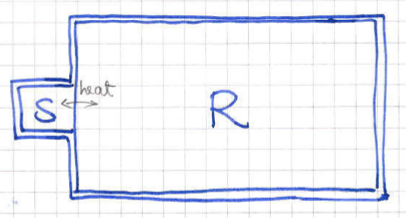
In this setup, at any given time we can define the energy the $E_S$ of our system $R$ and the energy $E_R\gg E_S$ of the reservoir. Since the system is interacting, each one of them is not separately conserved but as whole, the system $S\cup R$ can be thought of as an isolated system and therefore the total energy

$E_{tot}=E_S+E_R,$ (1)

is conserved and fixed. Moreover, with the system $R$ being large, we know that small small changes in $E_R$ will not alter the temperature $T_R$ of the reservoir, due to its large heat capacity $C_R$. In thermodynamic equilibrium we will have the the temperature $T_S$ of $S$ will be equal to that of the reservoir and

$T_S=T_R=T.$ (2)

Figure 2: Energy levels of a quantised system

1.1.1 The Quantum Canonical Ensemble

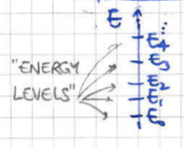
For simplicity, we will consider the case where both systems are quantum mechanical and whose microstates form a discrete set (they are quantised) as in figure 2. In general, for each energy level $E_n$ we can have $\mathrm{\Omega }(E_n)$ different microstates. This suggests that we can denote the microstates by $\mid n,i⟩$ with $i=1,\mathrm{\dots },\mathrm{\Omega }(E_n)$ and for each one the corresponding energy would be $E_n$. To keep our notation simple we will simply use the energy level index i.e. $\mid n⟩$.

Since $E_S$ is not fixed, the natural question to ask is “What is the probability $p_n$ for the system $S$ to be in a given microstate $\mathrm{\mid }n\mathrm{⟩}$ of energy $E_S\mathrm{=}{E}_n$?”. In order to answer this, we will exploit the fact that the total system $S\cup R$ is in the microcanonical ensemble. According to Boltzmann’s of equal a priori probabilities for $S\cup R$, all states of $S\cup R$ with total energy $E_{tot}$ are of equal probability. The task is then to count how many microstates ${\mathrm{\Omega }}_{S\cup R}$ of the total system are compatible having total energy $E_{tot}$ for any given microstate $\mid n⟩$ of $S$.

We will call ${\mathrm{\Omega }}_R(E_R)$ the number of microstates of the reservoir $R$ corresponding to energy $E_R=E_{tot}-E_n$. Correspondingly, we will call ${\mathrm{\Omega }}_S(E_n)$ the number of microstates of $S$ corresponding to energy $E_n$. If we fix a particular state $\mid n⟩$ of $S$, we can then see that we have a total of ${\mathrm{\Omega }}_{S\cup R}(\mid n⟩)={\mathrm{\Omega }}_R(E_{tot}-E_n)$ compatible microstates for the total system with the total system having fixed energy $E_{tot}$. From the microcanonical ensemble we now recall the Boltzmann entropy

$S_R(E_R)=k_B\ln \mathrm{\Omega }(E_R),$ (3)

for the reservoir $R$. Moreover using the fact that $E_n\ll E_{tot}$, we can perform a Taylor expansion to approximate,

$S_R(E_R)$ $=S_R(E_{tot}-E_n)\approx S_R(E_{tot})-E_n{\displaystyle \frac{\partial }{\partial E_{tot}}}{S}_R(E_{tot})$

$=S_R(E_{tot})-{\displaystyle \frac{1}{T}}{E}_n,$ (4)

after using the definition of temperature

${\displaystyle \frac{1}{T}}={\displaystyle \frac{\partial S}{\partial E}}.$ (5)

We can now estimate the number of states we are after according to,

${\mathrm{\Omega }}_{S\cup R}(\mid n⟩)=e^{\frac{1}{k_B}{S}_R(E_{tot}-E_n)}\approx e^{\frac{1}{k_B}{S}_R(E_{tot})}{e}^{-\beta E_n},$ (6)

where we defined ${\beta }^{-1}=k_{B}T$. At this point we note that the number $e^{\frac{1}{k_B}{S}_R(E_{tot})}$ only depends on the properties of the reservoir $R$ which is independent of the microstate $\mid n⟩$ we are interested. In other words, it is just a constant independent of $\mid n⟩$.

Boltzamann’s principle of equal a priori probabilities (applied to $S\cup R$) gives the Boltzmann distribution,

$p(\mid n⟩)=Z^{-1}{e}^{-\beta E_n},$ (7)

where we have defined the temperature dependent normalisation constant

$Z={\displaystyle \sum _{\mid n⟩}}{e}^{-\beta E_n},$ (8)

also known as the Partition Function with the sum being over all microstates of $S$. Notice that all dependence on the reservoir $R$ has dropped out, or more precisely it is encoded in the temperature $T$ which is also the temperature of $S$.

Some important remarks about the partition function are

• The partition function $Z$ is defined as a simple normalisation factor in the Boltzmann distribution. However it will turn out to be the most fundamental object in Statistical Mechanics.

• The partition function is a function of $T$, $V$ and $N$.

• The Boltzmann weight $e^{-\frac{E_n}{k_{B}T}}$ favors microstates $\mid n⟩$ whose energy is .

Finally, we would like to comment on the case of combining two independent systems $A$ and $B$ held at tempterature $T$ with Hamiltonians $H_A$ and $H_B$. The total Hamiltonian is $H=H_A+H_B$ with no interaction term between the two systems. In this case, the total energy is $E_{tot}=E_A+E_B$ and the partition function of the combined system is given by summing over the microstates $\mid n_A⟩$ and $\mid n_B⟩$,

$Z_{tot}={\displaystyle \sum _{n_A,n_B}}{e}^{-\beta (E_{n_A}+E_{n_B})}=\left({\displaystyle \sum _{n_A}}{e}^{-\beta E_{n_A}}\right)\left({\displaystyle \sum _{n_B}}{e}^{-\beta E_{n_B}}\right)=Z_A{Z}_B.$ (9)

Therefore, for combinations of non-interacting systems the partition function of the total system is equal to the product of the partition functions of its sub-systems.

1.1.2 The Two State System

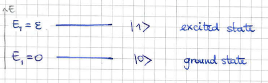
As an example, we will consider a quantum system which only has two possible microstates, corresponding to $n=0$ (the ground state $\mid 0⟩$) and $n=1$ (the excited state $\mid 1⟩$) with corresponding energies $E_0=0$ and $E_1=\epsilon$.

Figure 3: The energy levels of a two state quantum system

For this $N=1$ particle system the partition function (8) is

$Z_1$ $={\displaystyle \sum _n}{e}^{-\beta E_n}=e^{-\beta E_0}+e^{-\beta E_1}=1+e^{-\beta \epsilon }$

$=2e^{-\beta \epsilon /2}\cosh \left({\displaystyle \frac{\beta \epsilon }{2}}\right).$ (10)

The probabilities (7) of being in either state are

$p_{N=1,T}(0)={\displaystyle \frac{1}{1+e^{-\beta \epsilon }}},p_{N=1,T}(1)={\displaystyle \frac{e^{-\beta \epsilon }}{1+e^{-\beta \epsilon }}}.$ (11)

This allows us to compute the expectation value for the energy according to

${⟨E⟩}_{N=1}$ $=E_0{p}_{N=1,T}(0)+E_1{p}_{N=1,T}(1)=\epsilon {\displaystyle \frac{e^{-\beta \epsilon }}{1+e^{-\beta \epsilon }}}$

$={\displaystyle \frac{\epsilon }{2}}\left(1-\tanh \left({\displaystyle \frac{\beta \epsilon }{2}}\right)\right).$ (12)

If we now consider $N$ distinguishable copies of the two state system, the partition function is

$Z_N=Z_1^N=2^N{e}^{-N\beta \epsilon /2}{\cosh }^N\left({\displaystyle \frac{\beta \epsilon }{2}}\right).$ (13)

For the combined system, the possible microstates are labelled by an $N$ dimensional array $\overrightarrow{n}=(n_1,n_2,\mathrm{\dots },n_N)$ with $n_i=\pm 1$ for $i=1,\mathrm{\dots },N$. The corresponding energy for will then be

$E_{\overrightarrow{n}}={\displaystyle \sum _{i=1}^N}{n}_i{E}_{n_i}=N_1\epsilon$ (14)

where $N_1$ is the number of $n_i$’s which are equal to one. The corresponding probability is give by

$p_{N,T}(\overrightarrow{n})=Z_N^{-1}{e}^{-\beta E_{\overrightarrow{n}}}={\displaystyle \frac{e^{-N_1\beta \epsilon }}{{\left(1+e^{-\beta \epsilon }\right)}^N}}.$ (15)

To compute the expectation value of the energy we have to sum over all possible vectors $\overrightarrow{n}$,

${⟨E⟩}_N$ $={\displaystyle \sum _{\overrightarrow{n}}}{E}_{\overrightarrow{n}}{p}_{N,T}(\overrightarrow{n})={\displaystyle \sum _{N_1}^N}\left({\displaystyle \genfrac{}{}{0pt}{}{N}{N_1}}\right)N_1\epsilon {\displaystyle \frac{e^{-N_1\beta \epsilon }}{{\left(1+e^{-\beta \epsilon }\right)}^N}}=$

$={\displaystyle \frac{1}{{\left(1+e^{-\beta \epsilon }\right)}^N}}{\displaystyle \sum _{N_1}^N}\left({\displaystyle \genfrac{}{}{0pt}{}{N}{N_1}}\right)N_1\epsilon e^{-N_1\beta \epsilon }$

$=-{\displaystyle \frac{1}{{\left(1+e^{-\beta \epsilon }\right)}^N}}{\displaystyle \frac{\partial }{\partial \beta }}\left({\displaystyle \sum _{N_1}^N}\left({\displaystyle \genfrac{}{}{0pt}{}{N}{N_1}}\right)e^{-N_1\beta \epsilon }\right)$

$=-{\displaystyle \frac{1}{{\left(1+e^{-\beta \epsilon }\right)}^N}}{\displaystyle \frac{\partial }{\partial \beta }}{\left(1+e^{-\beta \epsilon }\right)}^N$

$=-{\displaystyle \frac{\partial }{\partial \beta }}\ln Z_N=-N{\displaystyle \frac{\partial }{\partial \beta }}\ln Z_1=N{⟨E⟩}_{N=1}$

$=N{\displaystyle \frac{\epsilon }{2}}\left(1-\tanh \left({\displaystyle \frac{\beta \epsilon }{2}}\right)\right).$ (16)

One can now make the following remarks

• The fact that ${⟨E⟩}_N=N{⟨E⟩}_{N=1}$ even for a small number of particles is related to the fact that we dealing with a non-interacting system and that energy is an extensive quantity.

• In the fifth line of the above derivation we noticed that the expectation value $⟨E⟩$ is related to the derivative of the logarithm of the partition function. This is not a coincidence particular to the case under consideration but a general statement we will later prove.

1.1.3 The Classical Canonical Ensemble (Distinguishable Particles)

As we saw in the quantum case of section 1.1.1, the first step is to count how many microstates of the reservoir $R$ are compatible with the total energy condition

$E_{tot}=E_S+E_R,$ (17)

given a specific microstate of $S$. Therefore, the basic logic in counting states in the classical version of the canonical ensemble is identical the quantum one. As you have already seen in the microcanonical ensemble, the number of classical states ${\mathrm{\Omega }}_R(E_R)$ can be found by computing the area of the phase space hypersurface

${𝒩}_R(E_R)={\displaystyle {\int }_{{𝒫}_R}}𝑑q_R𝑑p_R\delta (H_R(p_R,q_R)-E_R).$ (18)

The number of states then is given by

${\mathrm{\Omega }}_R(E_R)={\displaystyle \frac{{𝒩}_R(E_R)}{{𝒩}_0}},$ (19)

where ${𝒩}_0=h^S$ is the phase space area per classical state and $h$ has dimensions $[momentum]\times [length]=[energy]\times [time]$. This is a very awkward step that we will derive it later in the term when we derive the classical partition from the quantum one. There we will show that the mysterious constant $h$ is nothing but Planck’s constant.The number $S$ is the number of degrees of freedom of our phase system. Another important point is that formula (18) assumes that the particles are distinguishable. This is perfectly fine with the classical laws of physics as we can attach labels to each particle and keep track of them during their whole time evolution. However, we will see in a later section that this is going to be problematic in the context of statistical mechanics.

After these remarks, we can follow all the steps that we of the quantum case to show that the probability density of a classical microstate of $S$ labelled by position coordinates $q$ and momentum coordinates $p$ to occur is,

$p_{T,V,N}(q_j,p_j)=Z^{-1}{e}^{-\beta H(q_j,p_j)}.$ (20)

Once again, we have discovered the Boltzmann distribution. The dimensionless partition function $Z$ in the classical case is

$Z={\displaystyle {\int }_{𝒫}}\left({\displaystyle \prod _{i=1}^S}{\displaystyle \frac{d{q}_{i}d{p}_i}{h}}\right)e^{-\beta H(q_j,p_j)}.$ (21)

Note that when we write the above formula, we are summing over all inequivalent particle configurations. The above is correct as long as the particles are distinguishable.

The Boltzmann distribution (20) can be used to compute the probability $P_{T,V,N}(ℬ)$ for the system to be in a microstate in $ℬ\subset 𝒫$. In our conventions we have

$P_{T,V,N}(ℬ)={\displaystyle {\int }_{ℬ}}\left({\displaystyle \prod _{i=1}^S}{\displaystyle \frac{d{q}_{i}d{p}_i}{h}}\right)p_{T,V,N}(q_j,p_j).$ (22)

1.1.4 Energy And Fluctuations

Given our current understanding, we can now link the microscopic description of our system to thermodynamic quantities concerning the macroscopic world. This time to make the discussion simpler we will start from the classical case. Given a physical quantity $A(q_i,p_j)$, it is meaningful to consider its expectation value,

$⟨A⟩={\displaystyle {\int }_{𝒫}}\left({\displaystyle \prod _{i=1}^S}{\displaystyle \frac{d{q}_{i}d{p}_i}{h}}\right)A(q_j,p_j)p_{T,V,N}(q_j,p_j).$ (23)

In the case of the microcanonical ensemble, the total energy $E$ of the system is fixed. However, in the case of the macrocanonical ensemble we keep the temperature $T$ fixed. Therefore, since the energy fluctuates, it makes perfect sense to consider its expectation value by computing $⟨E⟩=⟨H⟩$ through equation (23). Using the Boltzmann distribution (20) we now see that

$⟨E⟩$ $={\displaystyle \frac{1}{Z}}{\displaystyle {\int }_{𝒫}}\left({\displaystyle \prod _{i=1}^S}{\displaystyle \frac{d{q}_{i}d{p}_i}{h}}\right)H(q_j,p_j)e^{-\beta H(q_j,p_j)}$

$=-{\displaystyle \frac{1}{Z}}{\displaystyle \frac{\partial }{\partial \beta }}\left({\displaystyle {\int }_{𝒫}}\left({\displaystyle \prod _{i=1}^S}{\displaystyle \frac{d{q}_{i}d{p}_i}{h}}\right)e^{-\beta H(q_j,p_j)}\right)$

$=-{\displaystyle \frac{1}{Z}}{\displaystyle \frac{\partial }{\partial \beta }}Z\Rightarrow$

$⟨E⟩$ $=-{\displaystyle \frac{\partial }{\partial \beta }}\ln Z,$ (24)

where in the third line we used the definition (21). This is one of the profound results of statistical mechanics linking thermodynamic quantities to the Hamiltonian of a system via the partition function $Z$.

In order to prove the same result for a quantum mechanical system need to consider the discrete version of Boltzmann’s distribution (7) to write

$⟨E⟩$ $={\displaystyle \sum _{\mid n⟩}}{E}_n{p}_n={\displaystyle \frac{1}{Z}}{\displaystyle \sum _{\mid n⟩}}{E}_n{e}^{-\beta E_n}$

$=-{\displaystyle \frac{1}{Z}}{\displaystyle \frac{\partial }{\partial \beta }}\left({\displaystyle \sum _{\mid n⟩}}{e}^{-\beta E_n}\right)$

$=-{\displaystyle \frac{1}{Z}}{\displaystyle \frac{\partial }{\partial \beta }}Z\Rightarrow$

$⟨E⟩$ $=-{\displaystyle \frac{\partial }{\partial \beta }}\ln Z.$ (25)

This time we used the quantum version of the definition of the partition function in equation (8).

Another statistical quantity we would like to consider is the variance

${\sigma }_E^2=⟨E^2⟩-{⟨E⟩}^2.$ (26)

For any integer $n>0$ we can write,

$⟨E^n⟩$ $={\displaystyle \frac{1}{Z}}{\displaystyle {\int }_{𝒫}}\left({\displaystyle \prod _{i=1}^S}{\displaystyle \frac{d{q}_{i}d{p}_i}{h}}\right)H^n(q_j,p_j)e^{-\beta H(q_j,p_j)}$

$={(-)}^n{\displaystyle \frac{1}{Z}}{\displaystyle \frac{{\partial }^n}{\partial {\beta }^n}}\left({\displaystyle {\int }_{𝒫}}\left({\displaystyle \prod _{i=1}^S}{\displaystyle \frac{d{q}_{i}d{p}_i}{h}}\right)e^{-\beta H(q_j,p_j)}\right)$

$={(-)}^n{\displaystyle \frac{1}{Z}}{\displaystyle \frac{{\partial }^n}{\partial {\beta }^n}}Z.$ (27)

Setting $n=2$ we have,

${\sigma }_E^2$ $={\displaystyle \frac{1}{Z}}{\displaystyle \frac{{\partial }^2}{\partial {\beta }^2}}Z-{\displaystyle \frac{1}{Z^2}}{\left({\displaystyle \frac{\partial }{\partial \beta }}Z\right)}^2$

$={\displaystyle \frac{\partial }{\partial \beta }}\left({\displaystyle \frac{1}{Z}}{\displaystyle \frac{\partial }{\partial \beta }}Z\right)$

$={\displaystyle \frac{{\partial }^2}{\partial {\beta }^2}}\ln Z=-{\displaystyle \frac{\partial }{\partial \beta }}⟨E⟩.$ (28)

Similarly to the case of the microcanonical ensemble, we can define the heat capacity

$C_{V,N}={\displaystyle \frac{\partial }{\partial T}}⟨E⟩.$ (29)

After using the chain rule we have the revealing relation,

$C_{V,N}={\displaystyle \frac{\partial \beta }{\partial T}}{\displaystyle \frac{\partial }{\partial \beta }}⟨E⟩={\displaystyle \frac{1}{k_B{T}^2}}{\sigma }_E^2,$ (30)

or equivalently

${\sigma }_E^2=k_B{T}^2{C}_{V,N}.$ (31)

This equation relates a statistical quantity describing the microscopic fluctuations of the energy to the heat capacity, a thermodynamic one that can be measured macroscopically. This relation is an example of a much more general result known as the fluctuation - dissipation theorem.

With the energy $⟨E⟩$ being an extensive quantity, we can argue that in the thermodynamic limit with $N\to \mathrm{\infty }$ we must have $⟨E⟩\propto N$ and therefore $C_{V,N}\propto N$ since temperature is an intensive quantity. Equation (31) then suggests that ${\sigma }_E\propto \sqrt{N}$ and

${\displaystyle \frac{{\sigma }_E}{⟨E⟩}}\propto {\displaystyle \frac{1}{\sqrt{N}}}\to 0,$ (32)

as a consequence of the central limit theorem. This shows that in the thermodynamic limit the canonical and microcanonical ensembles coincide.

1.1.5 Entropy

In the case of the microcanonical ensemble the entropy is given by Boltzmann’s formula

$S=k_B\ln \mathrm{\Omega },$ (33)

in terms of the number of inequivalent microstates $\mathrm{\Omega }(E)$ of energy $E$.

We can now try follow Gibbs’ argument in order to understand entropy in way that would be applicable to the case of the canonical ensemble. We consider a large number $W$ of indistinguishable copies of our system. We now want to count the inequivalent ways of partitioning our $W$ systems in $W_1$ systems in the state $\mid 1⟩$, $W_2$ systems in the state $\mid 2⟩$ and so on so that ${\sum }_i{W}_i=W$. The number of inequivalent partitions is given by the multinomial coefficient,

$\mathrm{\Omega }={\displaystyle \frac{W!}{{\prod }_i{W}_i!}}.$ (34)

When we consider a large number of systems systems obeying a particular probability distribution $p(i)$, we expect that they will be distributed according to $W_i=p(i)W$. The total entropy is then,

$S_W$ $=k_B\ln \mathrm{\Omega }\approx k_B\left[W\ln W-{\displaystyle \sum _{\mid n⟩}}p(\mid n⟩)W\ln \left(p(\mid n⟩)W\right)\right]$

$=-W{k}_B{\displaystyle \sum _{\mid n⟩}}p(\mid n⟩)\ln p(\mid n⟩),$ (35)

where we used Stirling’s approximating formula. From the above we see that to each copy of our system we can associate an entropy

$S$ $=-k_B{\displaystyle \sum _{\mid n⟩}}p(\mid n⟩)\ln p(\mid n⟩)$

$=-k_B⟨\ln p⟩.$ (36)

We have arrived at a very general formula which depends solely on the distribution of the ensemble. As we will see later, one can arrive arrive at the probability distributions of both the microcanonical and the canonical ensembles by simply demanding the extremisation of the Gibbs entropy (1.1.5).

We will now apply the entropy formula (1.1.5) for the two ensembles we have considered so far.

• The Microcanonical Ensemble:

  We consider a system at fixed energy $E$. The probability distribution is such that

  (37)

  In order to apply (1.1.5) we need to sum over all states

  $S$ $=-k_B{\displaystyle \sum _{\mid n⟩}}p(\mid n⟩)\ln p(\mid n⟩)$

  $=-k_B\mathrm{\Omega }(E){\displaystyle \frac{1}{\mathrm{\Omega }(E)}}\ln {\displaystyle \frac{1}{\mathrm{\Omega }(E)}}$

  $=k_B\ln \mathrm{\Omega }(E),$ (38)

  which agree with the Boltzmann entropy for the microcanonical ensemble as we would expect.

• The Canonical Ensemble:

  For the canonical ensemble we will use the Boltzmann distribution (7) at a fixed temperature $T$. Summing over all microstates we have

  $S$ $=-{\displaystyle \frac{k_B}{Z}}{\displaystyle \sum _{\mid n⟩}}{e}^{-\beta E_n}\ln \left({\displaystyle \frac{e^{-\beta E_n}}{Z}}\right)$

  $={\displaystyle \frac{\beta k_B}{Z}}{\displaystyle \sum _{\mid n⟩}}{E}_n{e}^{-\beta E_n}+{\displaystyle \frac{k_B\ln Z}{Z}}{\displaystyle \sum _{\mid n⟩}}{e}^{-\beta E_n}$

  $=\beta k_B{\displaystyle \sum _{\mid n⟩}}{E}_n{\displaystyle \frac{e^{-\beta E_n}}{Z}}+{\displaystyle \frac{k_B\ln Z}{Z}}{\displaystyle \sum _{\mid n⟩}}{e}^{-\beta E_n}$

  $=\beta k_B{\displaystyle \sum _{\mid n⟩}}{E}_{n}p(\mid n⟩)+k_B\ln Z$

  $=\beta k_B⟨E⟩+k_B\ln Z$

  $=-\beta k_B{\displaystyle \frac{\partial }{\partial \beta }}\ln Z+k_B\ln Z$

  $=k_{B}T{\displaystyle \frac{\partial }{\partial T}}\ln Z+k_B\ln Z$

  $=k_B{\displaystyle \frac{\partial }{\partial T}}\left(T\ln Z\right)\Rightarrow$

  $S$ $=k_B{\displaystyle \frac{\partial }{\partial T}}\left(T\ln Z\right).$ (39)

  In the fourth line we used once again equation (7) and the definition of the partition function (8). In the sixth line we used the fact that the energy average can be found from (1.1.4). Once again, we see that the partition function is much more than just a normalisation constant in the Boltzmann distribution.

1.1.6 Transgression: Entropy Extremising Distributions

One of the most fundamental ideas in this course is that the thermodynamic entropy is given by the number of inequivalent occurrences of a system after having fixed a probability distribution. We have seen that the principle of a priori equal probabilities of microstastes in Statistical Mechanics fixes those probability distributions in the microcanonical and canonical ensembles.

We now want to reverse the question. Suppose that we take the definition of entropy (1.1.5) for granted. The question we want to ask is how would then the principles of thermodynamics on entropy fix the probability distributions for us? We will pretend that we don’t know what the microstate probabilities $p(\mid n⟩)$ are and that all we know is that they should be such that the entropy (1.1.5) is maximised and that they should satisfy constraints compatible with the macroscopic/thermodynamic properties of the system.

The task for each ensemble then is to extremise the Gibbs entropy with respect to $p(\mid n⟩)$ under the constraint,

${\displaystyle \sum _{\mid n⟩}}p(\mid n⟩)=1,$ (40)

and

• For the microcanonical ensemble with fixed energy $E$, we need to set $p(\mid n⟩)=0$ unless $E_n=E$.

• For the canonical ensemble we would need to fix the temperature. Instead of that we can equivalently demand that we fix the average energy

  $⟨E⟩={\displaystyle \sum _{\mid n⟩}}{E}_{n}p(\mid n⟩).$ (41)

As we know, in order to extremise a function under certain constraints we need to introduce Lagrange multipliers. For the case of the microcanonical ensemble we introduce the function,

$W$ $=S+\alpha \left({\displaystyle \sum _{\mid n⟩}}p(\mid n⟩)-1\right)$

$=-k_B{\displaystyle \sum _{\mid n⟩}}p(\mid n⟩)\ln p(\mid n⟩)+\alpha \left({\displaystyle \sum _{\mid n⟩}}p(\mid n⟩)-1\right),$ (42)

where $\alpha$ is the Lagrange multiplier enforcing the constraint (40). After introducing the Lagrange multiplier $\alpha$ we can now extremise the function $W$ by demanding,

${\displaystyle \frac{\partial }{\partial p(\mid m⟩)}}W$ $=0\Rightarrow$

$-k_B\left(\ln p(\mid n⟩)+1\right)+\alpha$ $=0\Rightarrow$

$p(\mid n⟩)$ $=e^{k_B^{-1}\alpha -1},$ (43)

which does not depend on the state, as long as the state satisfies the macroscopic constraint $E_n=E$. We therefore see that extremisation of the entropy is equivalent to Boltzmann’s principle of a priori equal probabilities. In order to fix the constant $\alpha$ that appears in the expression for the probabilities,we now examine the constraint,

${\displaystyle \sum _{\mid n⟩}}p(\mid n⟩)=1\Rightarrow {\displaystyle \sum _{\begin{array}{c}\mid n⟩\mathrm{with}\\ E_n=E\end{array}}}p(\mid n⟩)$ $=1\Rightarrow$ (46)

${\displaystyle \sum _{\begin{array}{c}\mid n⟩\mathrm{with}\\ E_n=E\end{array}}}{e}^{k_B^{-1}\alpha -1}=1\Rightarrow \mathrm{\Omega }(E)e^{k_B^{-1}\alpha -1}$ $=1\Rightarrow$ (49)

$e^{k_B^{-1}\alpha -1}={\displaystyle \frac{1}{\mathrm{\Omega }(E)}}.$ (50)

From the above we recover our familiar

(51)

We will leave the case of the microcanonical ensemble as an exercise.

1.1.7 Most Likely vs Average Energy

In this subsection we want to discuss the probability $p(E_n)$ for energy levels instead of specific microstates within the canonical ensemble. Given that all $\mathrm{\Omega }(E_n)$ microstates of energy $E_n$ have the same probability, we have

$p(E_n)$ $={\displaystyle \sum _{\begin{array}{c}\mid m⟩\mathrm{with}\\ E_m=E_n\end{array}}}p(\mid m⟩)$ (54)

$={\displaystyle \frac{1}{Z}}\mathrm{\Omega }(E_n)e^{-\beta E_n}.$ (55)

After using the Boltzmann entropy for the energy level $E_n$ we have

$p(E_n)$ $={\displaystyle \frac{1}{Z}}{e}^{-\beta E_n+\frac{1}{k_B}{S}_B(E_n)}$

$={\displaystyle \frac{1}{Z}}{e}^{-\beta \left(E_n-T{S}_B(E_n)\right)}.$ (56)

Correspondingly, the partition function can be written as

$Z$ $={\displaystyle \sum _{\mid n⟩}}{e}^{-\beta E_n}$

$={\displaystyle \sum _{E_n}}{e}^{-\beta \left(E_n-T{S}_B(E_n)\right)}.$ (57)

where we used the definition of the Boltzmann entropy associated to each of the energy levels $E_n$.

The most probable energy level $E_{\ast }=E_n$ is specified by minimising $E_n-TS(E_n)$ with respect to $E_n$. This gives us

${{\displaystyle \frac{\partial }{\partial E_n}}\left(E_n-T{S}_B(E_n)\right)|}_{E_n=E_{\ast }}$ $=0$

$1-{T{\displaystyle \frac{\partial }{\partial E_n}}{S}_B(E_n)|}_{E_n=E_{\ast }}$ $=0$

$1-{{\displaystyle \frac{T}{T(E_n)}}|}_{E_n=E_{\ast }}$ $=0$

$1-{\displaystyle \frac{T}{T(E_{\ast })}}$ $=0$

$T(E_{\ast })$ $=T.$ (58)

Inverting the last equation then fixes $E_{\ast }=E_{\ast }(\beta )$. In the third line we used the definition of temperature $T_n$ associated to the $n$-th energy level according to the microcanonical ensemble. This is of course in general different from the temperature $T$ that we hold our system in the canonical ensemble. However, we see that the most likely energy level is the one whose microcanonical temperature $T(E_{\ast })$ is equal to $T$.

The important point of this computation is that the free energy,

$F(E_n)=E_n-T{S}_B(E_n),$ (59)

is minimised for a macroscopic system at fixed $T$, $V$ and $N$. We will see much more about this quantity from a thermodynamics point of view in the next subsection. We can see that this is achieved through a competition between,

• Minimising energy $E$ (”energy minimisation”) which wins at low $T$,

• Maximising degeneracy through $S(E)$ (”entropy maximisation”) which wins at high $T$.

In the thermodynamic limit with $⟨E⟩,S\propto N\to \mathrm{\infty }$, the partition function (1.1.7) is determined by the largest term which is also the term with $E_n=E_{\ast }$. We therefore have,

$Z\approx \mathrm{\Omega }(E_{\ast }(\beta ))e^{-\beta E_{\ast }(\beta )}=e^{-\beta \left(E_{\ast }(\beta )-T{S}_B(E_{\ast }(\beta ))\right)}.$ (60)

At this point, it is worth using the above thermodynamic limit approximation to compute the average energy,

$⟨E⟩$ $=-{\displaystyle \frac{\partial }{\partial \beta }}\ln Z$

$\approx -{\displaystyle \frac{\partial }{\partial \beta }}\left(\mathrm{\Omega }(E_{\ast }(\beta ))e^{-\beta E_{\ast }(\beta )}\right)$

$={\displaystyle \frac{\partial }{\partial \beta }}\left(\beta E_{\ast }(\beta )-{\displaystyle \frac{1}{k_B}}{S}_B(E_{\ast }(\beta ))\right)$

$=E_{\ast }(\beta )+{{\displaystyle \frac{1}{k_B}}\left({\displaystyle \frac{1}{T}}-{\displaystyle \frac{\partial }{\partial E_n}}{S}_B(E_n)\right)|}_{E_n=E_{\ast }}{\displaystyle \frac{\partial }{\partial \beta }}{E}_{\ast }(\beta )$

$=E_{\ast }(\beta ).$ (61)

In the penultimate line, the bracket equal to zero due to equation (1.1.7) that $E_{\ast }$ satisfies. We therefore see that in the thermodynamic limit:

• The average energy is also equal to the most likely energy level to occur.

• The ratio ${\sigma }_E/⟨E⟩$ goes to zero.

Another interesting quantity we can compute in the thermodynamic limit is the entropy (• ‣ 1.1.5). We can write

$S$ $=k_B{\displaystyle \frac{\partial }{\partial T}}\left(T\ln Z\right)$

$=k_B\left(1-\beta {\displaystyle \frac{\partial }{\partial \beta }}\right)\ln Z$

$=\left(k_B\ln Z+k_B\beta ⟨E⟩\right)$

$=\left(S_B(E_{\ast }(\beta ))+k_B\beta \left(⟨E⟩-E_{\ast }(\beta )\right)\right)$

$=S_B(E_{\ast })=k_B\ln \mathrm{\Omega }(E_{\ast }),$ (62)

where we used the expression (1.1.4) for the average energy $⟨E⟩$. We therefore see that in the limit we are interested in, the Gibbs entropy of the canonical distribution coincides with the Boltzmann entropy of the most likely energy level.

1.1.8 The Free Energy

In the canonical ensemble we define the free energy to be,

$F=⟨E⟩-TS,$ (63)

which by construction is a function of $T$, $V$ and $N$. More generally, independently of the thermodynamic limit we can use equation (• ‣ 1.1.5) to write

$S$ $=k_B{\displaystyle \frac{\partial }{\partial T}}\left(T\ln Z\right)$

$=k_B\left(1-\beta {\displaystyle \frac{\partial }{\partial \beta }}\right)\ln Z$

$=\left(k_B\ln Z+k_B\beta ⟨E⟩\right).$ (64)

The free energy (63) then reads

$F$ $=⟨E⟩-TS$

$=-k_{B}T\ln Z,$ (65)

and we see another instance where the partition function fixes a macroscopic quantity. Notice that we can invert this relation to express the partition function in terms of the free energy of the system,

$Z=e^{-\beta F}.$ (66)

One might wonder why is the free energy (63) important? In the previous subsection 1.1.7 we saw that in the thermodynamic limit, the energy level that extremises this quantity is the most likely one. From a thermodynamics point of view, it is the appropriate thermodynamic potential when considering systems at fixed temperature, volume and particle number.

To see this, notice that the Gibbs entropy (• ‣ 1.1.5) simply a partial derivative of the free energy with respect to temperature,

$S=-{\displaystyle \frac{\partial F}{\partial T}}.$ (67)

Apart from this, the First law of thermodynamics,

$dE=TdS-pdV+\mu dN,$ (68)

where we have included the definition of the chemical potential as the change in energy when we increase the number of particles at fixed entropy and volume. This quantity will become very important to us later when we discuss the grand canonical ensemble. The first law then lets us write the differential of the free energy as,

$dF$ $=dE-TdS-SdT$

$=-SdT-pdV+\mu dN,$ (69)

from which we can clearly see that it is a function of $T$, $V$ and $N$ and therefore the most natural thermodynamic potential when these variables are fixed. Moreover, we can see that in addition to the entropy, we can extract the pressure and the chemical potential from the partial derivatives with respect to volume and particle number,

$S=-{\displaystyle \frac{\partial F}{\partial T}},p=-{\displaystyle \frac{\partial F}{\partial V}},\mu ={\displaystyle \frac{\partial F}{\partial N}}.$ (70)

As we already know, this is a general property of Legendre transformations. We started from the energy $E$ which has to be considered as a function of entropy $S$, volume $V$ and particle number $N$. In this language, the temperature is the derivative of energy with respect to entropy. The free energy (63) is simply the Legendre transformation which trades $S$ for $T$ which is the partial derivative of $E$ with respect to $S$.

1.2 The Grand Canonical Ensemble

When we moved from the microcanonical ensemble to the canonical, we dropped the idea of an energetically closed system. More specifically, we brought the system $S$ in thermal contact with a reservoir $R$ and thermodynamic equilibrium implied that the two systems would have to have the temperature $T$.

We will do something very similar in the case of the grand canonical ensemble with the extra complication that $S$ and $R$ can also exchange particles. In parallel with the case of energy, the system $S$ can have particle number $N_S$ and the reservoir can have particle number $N_R$. Even though $N_S$ and $N_R$ are not separately conserved, the total particle number $N_{tot}=N_R+N_S$ is. In order to describe equilibrium in this case, it will be useful to introduce the notion of chemical potential.

1.2.1 The Chemical Potential

Suppose that we bring in thermal contact two systems $S_1$ and $S_2$ which are also allowed to exchange particles. The total system $S=S_1\cup S_2$ can be considered to be in the microcanonical ensemble with fixed total energy $E_{tot}=E_1+E_2$, particle number $N_{tot}=N_1+N_2$ and volume.

Since $E_i$ and $N_i$ are allowed to fluctuate, a natural question to ask is what is the most likely partition of energy and particle number between the two systems. In order to do this, we need to ask how many microstates ${\mathrm{\Omega }}_S(E_1,E_2,N_1,N_2)$ does the total system have that would be compatible with this partition. This is a simple question in combinatorics and the answer is

${\mathrm{\Omega }}_S(E_1,E_2,N_1,N_2)={\mathrm{\Omega }}_1(E_1,N_1){\mathrm{\Omega }}_2(E_2,N_2),$ (71)

where ${\mathrm{\Omega }}_i$ is the number of microstates of the system $S_i$ at energy $E_i$ and particle number $N_i$. Alternatively, we can express this in terms of the Boltzmann entropies of the two systems according to

${\mathrm{\Omega }}_S(E_1,E_2,N_1,N_2)=e^{\frac{1}{k_B}\left(S_1(E_1,N_1)+S_2(E_2,N_2)\right)}.$ (72)

The principle of equal a priori probabilities would then tell us that the most likely partition would be the one that maximises ${\mathrm{\Omega }}_S$ under the constraints of fixed total energy and particle number.

In the case of only thermal contact, these considerations brought you to the discussion of temperature and the zeroth law of thermodynamics. This came about by extremising ${\mathrm{\Omega }}_S$ with respect to the partition of energy. In the present case, we will have to extremise with respect to both energy and particle number while retaining the constraints. We can write,

${\mathrm{\Omega }}_S(E_1,E_{tot},N_1,N_{tot})=e^{\frac{1}{k_B}\left(S_1(E_1,N_1)+S_2(E_{tot}-E_1,N_{tot}-N_1)\right)}$ (73)

and then extremise the exponent with respect to $E_1$ and $N_1$. Doing so, we obtain

$\begin{array}{cc}{\frac{\partial }{\partial E_1}\left(S_1(E_1,N_1)+S_2(E_{tot}-E_1,N_{tot}-N_1)\right)|}_{E_1=E_1^{\ast },N_1=N_1^{\ast }}=0\hfill & \\ {\frac{\partial }{\partial N_1}\left(S_1(E_1,N_1)+S_2(E_{tot}-E_1,N_{tot}-N_1)\right)|}_{E_1=E_1^{\ast },N_1=N_1^{\ast }}=0\hfill & \end{array}\}$ $\Rightarrow$ (76)

$\begin{array}{cc}{\frac{\partial }{\partial E_1}\left(S_1(E_1,N_1)+S_2(E_{tot}-E_1,N_{tot}-N_1)\right)|}_{E_1=E_1^{\ast },N_1=N_1^{\ast }}=0\hfill & \\ {\frac{\partial }{\partial N_1}\left(S_1(E_1,N_1)+S_2(E_{tot}-E_1,N_{tot}-N_1)\right)|}_{E_1=E_1^{\ast },N_1=N_1^{\ast }}=0\hfill & \end{array}\}$ $\Rightarrow$ (79)

$\begin{array}{cc}{\frac{\partial }{\partial E_1}{S}_1(E_1,N_1)|}_{E_1=E_1^{\ast },N_1=N_1^{\ast }}={\frac{\partial }{\partial E_2}{S}_2(E_2,N_2)|}_{E_2=E_2^{\ast },N_2=N_2^{\ast }}\hfill & \\ {\frac{\partial }{\partial N_1}{S}_1(E_1,N_1)|}_{E_1=E_1^{\ast },N_1=N_1^{\ast }}={\frac{\partial }{\partial E_2}{S}_2(E_2,N_2)|}_{E_2=E_2^{\ast },N_2=N_2^{\ast }}.\hfill & \end{array}\}$ (82)

The first line of the above system of equations is nothing but the zeroth law of thermodynamics after identifying

${\displaystyle \frac{1}{T}}={{\displaystyle \frac{\partial S}{\partial E}}|}_{V,N}.$ (83)

The second equation in (76) is telling us that in thermodynamic equilibrium, apart from $T$, there is another intensive quantity which is equal between the two systems which are in contact. This is the chemical potential $\mu$ defined through,

${\displaystyle \frac{\mu }{T}}=-{{\displaystyle \frac{\partial S}{\partial N}}|}_{V,N}.$ (84)

We see that every time we allow one of the extensive quantities to not be conserved in our system, there is a corresponding intensive one that stays fixed in thermodynamic equilibrium. In the case of the grand canonical ensemble, the quantities that we are going to keep fixed are the temperature $T$, the volume $V$ and the chemical potential $\mu$.

1.2.2 The Grand Canonical Partition Function

The discussion for the case of the grand canonical ensemble is in parallel with the philosophy we followed in section 1.1 for the canonical ensemble. The only difference is that now we will also allow the particle numbers $N_S$ and $N_R$ to vary while $N_R\gg N_S$.

Once again, we want to ask what is the probability for a specific microstate $\mid n⟩$ of $S$ to occur consisting of $N_S=N_n$ particles and energy $E_S=E_n$. Just like in the case of the canonical ensemble, the total number of compatible microstates of $S\cup R$ are ${\mathrm{\Omega }}_{S\cup R}(\mid n⟩)={\mathrm{\Omega }}_R(E_{tot}-E_n,N_{tot}-N_n)$. Once again, using the definition of Boltzmann entropy we have,

${\mathrm{\Omega }}_{S\cup R}(\mid n⟩)=e^{\frac{1}{k_B}{S}_R(E_{tot}-E_n,N_{tot}-N_n)}.$ (85)

We will now follow the same steps as in the canonical ensemble and expand

$S_R(E_{tot}-E_n,N_{tot}-N_n)=$ $S_R(E_{tot},N_{tot})$

$+$ ${{\displaystyle \frac{\partial }{\partial E_n}}{S}_R(E_{tot}-E_n,N_{tot}-N_n)|}_{E_n=0,N_n=0}{E}_n$

$+$ ${{\displaystyle \frac{\partial }{\partial N_n}}{S}_R(E_{tot}-E_n,N_{tot}-N_n)|}_{E_n=0,N_n=0}{N}_n$

$+$ $𝒪(E_n^2,N_n^2)$

$=$ $S_R(E_{tot},N_{tot})-{\displaystyle \frac{\partial }{\partial E_{tot}}}{S}_R(E_{tot},N_{tot})E_n-{\displaystyle \frac{\partial }{\partial N_{tot}}}{S}_R(E_{tot},N_{tot})N_n$

$=$ $S_R(E_{tot},N_{tot})-{\displaystyle \frac{1}{T}}{E}_n+{\displaystyle \frac{\mu }{T}}{N}_n.$ (86)

In the last line we used the definition of the chemical potential in equation (84). The principle of a priori equal probabilities and equation (85) then yield,

$p(\mid n⟩)={\displaystyle \frac{1}{𝒵}}{e}^{-\beta (E_n-\mu N_n)},$ (87)

with $𝒵$ a constant of normalisation for the probability distribution. The constant $𝒵$ is then

$𝒵={\displaystyle \sum _{\mid n⟩}}{e}^{-\beta (E_n-\mu N_n)},$ (88)

which is also known as the grand canonical partition function. As we will see later, the grand canonical partition function fixes all the macroscopic quantities we might wish to extract. This is in parallel to the partition function (8) in the case of the canonical ensemble.

Up to now we have been using notation which is appropriate for a quantum mechanical system. For a classical system, the concepts we have used in our derivation remain the same. More specifically, the microstates are going to be labelled by the particle number $N$ which is not fixed and the positions and momenta of our particles $(q_i,p_i)$ with $i=1,\mathrm{\dots },N$. The energy $E_S$ of the microstate is then given in terms of the N-body Hamiltonian according to $E_S=H_N(q_i,p_i)$. The analog of the distribution (87) is the density

$p_N(q_i,p_i)={\displaystyle \frac{1}{𝒵}}{e}^{-\beta (H_N(q_i,p_i)-\mu N)}.$ (89)

For the case of distinguishable particles the classical grand canonical partition function is,

$𝒵={\displaystyle \sum _N}{\displaystyle {\int }_{{𝒫}_N}}{\displaystyle \prod _{i=1}^{S_N}}{\displaystyle \frac{d{q}_{i}d{p}_i}{h}}{e}^{-\beta (H_N(q_i,p_i)-\mu N)},$ (90)

where ${𝒫}_N$ is the $N$-body phase space and $S_N$ the corresponding degrees of freedom.

As an aside, we note that the grand canonical probability distribution (87) can be derived by following the ideas of section 1.1.6 around the Gibbs entropy defined in equation (1.1.5). For the case of the grand canonical ensemble, the appropriate constraints are,

The first line makes sure that the collection of number $p(\mid n⟩)$ do indeed correspond constitute a probability distribution. The second and the third constraints are equivalent to fixing the temperature and the chemical potential of the system.

1.2.3 Thermodynamics at fixed $T$ and $\mu$

In this subsection we could follow the logic of subsections 1.1.4, 1.1.5 and 1.1.8 in order to relate interesting thermodynamic quantities to the grand canonical partition function of equation (87). In the grand canonical ensemble we keep fixed $T$, $N$ and $\mu$. From the point of view of thermodynamics, we know that energy $E$ can be considered as a function of entropy $S$, volume $V$ and particle number $N$. As we already know, the first law of thermodynamics reads,

$dE=TdS-pdV+\mu dN,$ (91)

and we note that

$T={{\displaystyle \frac{\partial E}{\partial S}}|}_{V,N},\mu ={{\displaystyle \frac{\partial E}{\partial N}}|}_{S,V}.$ (92)

The above implies that the natural potential to consider at fixed $T$ and $\mu$ is the double Legendre transformation,

$\mathrm{\Phi }$ $=E-\mu N-TS,$ (93)

which is known as the grand canonical potential. To see that $\mathrm{\Phi }$ only depends on $T$, $V$ and $\mu$ we compute the differential,

$d\mathrm{\Phi }=dE-Nd\mu -\mu dN-SdT-TdS,$ (94)

which in combination with the first law (91) gives,

$d\mathrm{\Phi }=-SdT-pdV-Nd\mu .$ (95)

From the above we read off,

$S=-{\displaystyle \frac{\partial \mathrm{\Phi }}{\partial T}},p=-{\displaystyle \frac{\partial \mathrm{\Phi }}{\partial V}},N=-{\displaystyle \frac{\partial \mathrm{\Phi }}{\partial \mu }},$ (96)

as we might had expected from an appropriate thermodynamic potential.

1.2.4 Thermodynamics from Statistical Mechanics

Given that we know the probability distribution of microstates, it is natural to identify $E=⟨E⟩$ and $N=⟨N⟩$ in order to make the connection between statistics and thermodynamics. The least obvious thermodynamic quantity to identify is the entropy $S$ which is conjectured to be given by the Gibbs entropy (1.1.5). Ultimately, we would like to obtain the grand canonical potential $\mathrm{\Phi }$ from a microscopic description.

We start by examining the Gibbs entropy (1.1.5) for which we can write,

$S$ $=-k_B{\displaystyle \sum _{\mid n⟩}}p(\mid n⟩)\ln p(\mid n⟩)$

$={\displaystyle \frac{k_B}{𝒵}}{\displaystyle \sum _{\mid n⟩}}{e}^{-\beta (E_n-\mu N_n)}\left(\beta \left(E_n-\mu N_n\right)+\ln 𝒵\right)$

$={\displaystyle \frac{k_B\beta }{𝒵}}\left({\displaystyle \sum _{\mid n⟩}}\left(E_n-\mu N_n\right)e^{-\beta (E_n-\mu N_n)}\right)+k_B\ln 𝒵$

$=-{\displaystyle \frac{k_B\beta }{𝒵}}{\displaystyle \frac{\partial }{\partial \beta }}\left({\displaystyle \sum _{\mid n⟩}}{e}^{-\beta (E_n-\mu N_n)}\right)+k_B\ln 𝒵$

$=-{\displaystyle \frac{k_B\beta }{𝒵}}{\displaystyle \frac{\partial }{\partial \beta }}𝒵+k_B\ln 𝒵$

$={\displaystyle \frac{k_{B}T}{𝒵}}{\displaystyle \frac{\partial }{\partial T}}𝒵+k_B\ln 𝒵$

$=k_B{\displaystyle \frac{\partial }{\partial T}}\left(T\ln 𝒵\right).$ (97)

In the step from the fourth to the fifth line we used equation (88). This result is very analogous to equation (• ‣ 1.1.5) of the canonical ensemble. Of course, in the present case, we have the grand canonical partition function appearing instead.

Notice that the third line in the derivation of (1.2.4) can be written in an alternative way which is suggestive. After using the form of the grand canonical probability distribution (87) we can write,

$S$ $={\displaystyle \frac{1}{T}}\left(⟨E⟩-\mu ⟨N⟩\right)+k_B\ln 𝒵\Rightarrow$

$\mathrm{\Phi }$ $=⟨E⟩-\mu ⟨N⟩-TS,$ (98)

from where we can read off the relation,

$\mathrm{\Phi }=-k_{B}T\ln 𝒵.$ (99)

Combining this result along with (1.2.4) we just recover,

$S=-{\displaystyle \frac{\partial \mathrm{\Phi }}{\partial T}}.$ (100)

which is the first of the thermodynamics relations in (96).

As a check of the third equation in (96) we can perform the direct computation

$⟨N⟩$ $={\displaystyle \sum _{\mid n⟩}}{N}_{n}p(\mid n⟩)={\displaystyle \frac{1}{𝒵}}{\displaystyle \sum _{\mid n⟩}}{N}_n{e}^{-\beta \left(E_n-\mu N_n\right)}$

$={\displaystyle \frac{1}{\beta 𝒵}}{\displaystyle \frac{\partial }{\partial \mu }}\left({\displaystyle \sum _{\mid n⟩}}{e}^{-\beta \left(E_n-\mu N_n\right)}\right)$

$={\displaystyle \frac{k_{B}T}{𝒵}}{\displaystyle \frac{\partial 𝒵}{\partial \mu }}=-{\displaystyle \frac{\partial \mathrm{\Phi }}{\partial \mu }},$ (101)

where in the last line we used the relation (99). For the average energy, we can use equations (93), (99) along with (100) to obtain,

$⟨E⟩$ $=-{\displaystyle \frac{\partial }{\partial \beta }}\ln 𝒵+\mu ⟨N⟩$

$={\displaystyle \frac{1}{\beta }}\left(-\beta {\displaystyle \frac{\partial }{\partial \beta }}+\mu {\displaystyle \frac{\partial }{\partial \mu }}\right)\ln 𝒵.$ (102)

1.2.5 Statistical Fluctuations

In this subsection we would like to see the convergence properties of the grand canonical distribution in the thermodynamics limit where $V\to \mathrm{\infty }$ with $\mu$ and $T$ fixed. In this limit we expect that the extensive quantities we do not fix will scale like the volume which is the only extensive quantity that we hold fix. This argument constraints the large volume behaviour of average energy and particle number according to,

$⟨N⟩$ $=Vf(T,\mu )+𝒪(V^0)$

$⟨E⟩$ $=Vg(T,\mu )+𝒪(V^0),$ (103)

where $f$ and $g$ are only functions of $T$ and $\mu$.

A good measure of the statistical fluctuations in our system is provided by the variance

${\sigma }_E^2$ $=⟨E^2⟩-{⟨E⟩}^2,$

${\sigma }_N^2$ $=⟨N^2⟩-{⟨E⟩}^2.$ (104)

In the previous subsection we managed to express the averages of energy $⟨E⟩$ and particle number $⟨N⟩$ in terms of the grand canonical partition function $𝒵$. Here, we will need to consider the higher moments $⟨E^m⟩$ and $⟨N^m⟩$ for any positive integer $m$. Starting from the particle number we have,

$⟨N^m⟩$ $={\displaystyle \sum _{\mid n⟩}}{N}_n^{m}p(\mid n⟩)={\displaystyle \frac{1}{𝒵}}{\displaystyle \sum _{\mid n⟩}}{N}_n^m{e}^{-\beta \left(E_n-\mu N_n\right)}$

$={\displaystyle \frac{1}{{\beta }^m}}{\displaystyle \frac{1}{𝒵}}{\displaystyle \frac{{\partial }^m}{\partial {\mu }^m}}\left({\displaystyle \sum _{\mid n⟩}}{e}^{-\beta \left(E_n-\mu N_n\right)}\right)$

$={\displaystyle \frac{1}{{\beta }^m}}{\displaystyle \frac{1}{𝒵}}{\displaystyle \frac{{\partial }^m}{\partial {\mu }^m}}𝒵.$ (105)

In order to obtain a similar result for the energy, we define the linear differential operator

$𝒟=-\beta {\displaystyle \frac{\partial }{\partial \beta }}+\mu {\displaystyle \frac{\partial }{\partial \mu }}=T{\displaystyle \frac{\partial }{\partial T}}+\mu {\displaystyle \frac{\partial }{\partial \mu }}.$ (106)

This allows us to write

$⟨E^m⟩$ $={\displaystyle \sum _{\mid n⟩}}{E}_{n}p(\mid n⟩)={\displaystyle \frac{1}{𝒵}}{\displaystyle \sum _{\mid n⟩}}{E}_n^m{e}^{-\beta \left(E_n-\mu N_n\right)}$

$={\displaystyle \frac{1}{𝒵}}{\left(-{\displaystyle \frac{\partial }{\partial \beta }}+{\displaystyle \frac{\mu }{\beta }}{\displaystyle \frac{\partial }{\partial \mu }}\right)}^m\left({\displaystyle \sum _{\mid n⟩}}{e}^{-\beta \left(E_n-\mu N_n\right)}\right)$

$={\displaystyle \frac{1}{𝒵}}{\left({\displaystyle \frac{1}{\beta }}𝒟\right)}^m\left({\displaystyle \sum _{\mid n⟩}}{e}^{-\beta \left(E_n-\mu N_n\right)}\right)$

$={\displaystyle \frac{1}{𝒵}}𝒵.$ (107)

After these results, we can now go back to the discussion of the variances (1.2.5). In order to compute the particle number variance, we will use equation (1.2.5) for $m=1,2$ to obtain,

${\sigma }_N^2$ $={\displaystyle \frac{1}{{\beta }^2}}{\displaystyle \frac{1}{𝒵}}{\displaystyle \frac{{\partial }^2}{\partial {\mu }^2}}𝒵-{\displaystyle \frac{1}{{\beta }^2}}{\displaystyle \frac{1}{{𝒵}^2}}{\left({\displaystyle \frac{\partial }{\partial \mu }}𝒵\right)}^2$

$={\displaystyle \frac{1}{{\beta }^2}}{\displaystyle \frac{\partial }{\partial \mu }}\left({\displaystyle \frac{1}{𝒵}}{\displaystyle \frac{\partial }{\partial \mu }}Z\right)$

$=k_{B}T{\displaystyle \frac{\partial ⟨N⟩}{\partial \mu }}.$ (108)

Similarly for the energy variance in (1.2.5) we obtain,

${\sigma }_E^2$ $={\displaystyle \frac{1}{𝒵}}{\left({\displaystyle \frac{1}{\beta }}𝒟\right)}^2𝒵-{\displaystyle \frac{1}{{𝒵}^2}}{\left({\displaystyle \frac{1}{\beta }}𝒟𝒵\right)}^2$

$={\displaystyle \frac{1}{\beta }}𝒟\left({\displaystyle \frac{1}{𝒵}}{\displaystyle \frac{1}{\beta }}𝒟𝒵\right)$

$={\displaystyle \frac{1}{\beta }}𝒟⟨E⟩$

$=-{\displaystyle \frac{\partial ⟨E⟩}{\partial \beta }}+{\displaystyle \frac{\mu }{\beta }}{\displaystyle \frac{\partial ⟨E⟩}{\partial \mu }}$

$=k_B{T}^2{\displaystyle \frac{\partial ⟨E⟩}{\partial T}}+k_{B}T\mu {\displaystyle \frac{\partial ⟨E⟩}{\partial \mu }}.$ (109)

In the first and the third lines we used equation (1.2.5) for $m=1,2$.

Now that we have the expressions (1.2.5) and (1.2.5) we can ask the question of what happens to the statistical fluctuations in the thermodynamic limit. Our discussion around equation (1.2.5) along with the results of equations (1.2.5) and (1.2.5) leads us to the conclusion that

${\sigma }_E\sim {\sigma }_N\sim \sqrt{V},$ (110)

and therefore

${\displaystyle \frac{{\sigma }_E}{⟨E⟩}}\sim {\displaystyle \frac{{\sigma }_N}{⟨N⟩}}\sim {\displaystyle \frac{1}{\sqrt{V}}}\to 0.$ (111)

We see that even though we might be fixing different quantities in the three statistical ensembles, they all describe the same physics in the thermodynamic limit with the corresponding statistical fluctuations becoming unimportant.

1.3 Relations Between Ensembles

We have seen that in the thermodynamic limit, the microcanonical, the canonical and the grand canonical ensembles all lead to the same description. In this subsection we will make the connection between the different ensembles manifest even without taking the limit. In order to do this quantitatively, we need to identify appropriate quantities for each ensemble. Table 1 outlines the correspondence we are going to establish.

Ensemble	Important Quantity
Microcanonical	Number of microstates $\mathrm{\Omega }(E,V,N)$
	$\updownarrow$
Canonical	Partition function $Z(T,V,N)$
	$\updownarrow$
Grand Canonical	Grand canonical partition function $𝒵(T,V,\mu )$

Table 1: The arrows outline the mapping between the different ensembles.

• Grand Canonical $\mathrm{\leftrightarrow }$ Canonical

  We start by showing the correspondence for the quantum mechanical case noting that the classical case is analogous. The canonical partition function can be written as,

  $Z(T,V,N)={\displaystyle \sum _{\mid n⟩\mathrm{with}{N}_n=N}}{e}^{-\beta E_n},$ (112)

  where $N_n$ is the particle number of the state $\mid n⟩$. This allows us to write the grand canonical partition function

  $𝒵(T,V,\mu )$ $={\displaystyle \sum _{\mid n⟩}}{e}^{-\beta (E_n-\mu N_n)}$

  $={\displaystyle \sum _N}{\displaystyle \sum _{\mid n⟩\mathrm{with}{N}_n=N}}{e}^{-\beta (E_n-\mu N_n)}$

  $={\displaystyle \sum _N}{\displaystyle \sum _{\mid n⟩\mathrm{with}{N}_n=N}}{e}^{-\beta (E_n-\mu N)}$

  $={\displaystyle \sum _N}\left(e^{\beta \mu N}{\displaystyle \sum _{\mid n⟩\mathrm{with}{N}_n=N}}{e}^{-\beta E_n}\right)$

  $={\displaystyle \sum _N}{e}^{\beta \mu N}Z(T,V,N)$

  $={\displaystyle \sum _N}{z}^{N}Z(T,V,N)\Rightarrow$

  $𝒵(T,V,\mu )$ $={\displaystyle \sum _N}{z}^{N}Z(T,V,N).$ (113)

  where in the fifth line we used equation (112) and we also defined the fugacity $z=e^{\mu \beta }$. Equation (• ‣ 1.3) is the equation defining the correspondence we promised earlier. Notice that we can also invert equation (• ‣ 1.3) to write,

  $Z(T,V,N)={{\displaystyle \frac{1}{N!}}{\displaystyle \frac{{\partial }^N𝒵}{\partial z^N}}|}_{z=0}.$ (114)

• Microcanonical $\mathrm{\leftrightarrow }$ Canonical

  In order to establish the correspondence between the microcanonical and the canonical ensembles, we will need to introduce the energy density of microstates $g(E)$. Upon integration between e.g. $E_1$ and $E_2>E_1$, this quantity will yield the number of microstates between $E_1$ and $E_2$. For the classical case, $g(E)$ coincides with $\mathrm{\Omega }(E)$ i.e.

  $g(E,V,N)={\displaystyle {\int }_{𝒫}}{\displaystyle \prod _{i=1}^S}{\displaystyle \frac{d{q}_{i}d{p}_i}{h}}\delta (E-H(q_i,p_i)).$ (115)

  For the quantum mechanical case, where the spectrum of energy is discrete $E=E_n$, the density of microstates is

  $g(E,V,N)={\displaystyle \sum _{\mid n⟩}}\delta (E-E_n)={\displaystyle \sum _{E_n}}\mathrm{\Omega }(E_n)\delta (E-E_n).$ (116)

  Indeed, integrating between $E_1$ and $E_2$ we obtain,

  ${\displaystyle {\int }_{E_1}^{E_2}}g(E,V,N)𝑑E=$ ${\displaystyle \sum _{E_n}}\mathrm{\Omega }(E_n){\displaystyle {\int }_{E_1}^{E_2}}\delta (E-E_n)𝑑E$

  $=$ (117)

  as we would expect.

  The density of microstates $g(E,V,N)$,carries the same information with the function $\mathrm{\Omega }(E,V,N)$ which is the interesting quantity of the microcanonical ensemble. In the present context, we can use it to connect the canonical to the microcanonical ensemble. For the quantum case we can write,

  $Z(T,V,N)$ $={\displaystyle \sum _{\mid n⟩}}{e}^{-\beta E_n}={\displaystyle \sum _{E_n}}\mathrm{\Omega }(E_n)e^{-\beta E_n}$

  $={\displaystyle \int 𝑑Eg(E,V,N)e^{-\beta E}}.$ (118)

  We see that the canonical partition function is the Laplace transform of the density of microstates. The same result is also true for the classical case. To see this, we can write

  $Z(T,V,N)$ $={\displaystyle {\int }_{𝒫}}{\displaystyle \prod _{i=1}^S}{\displaystyle \frac{d{q}_{i}d{p}_i}{h}}{e}^{-\beta H(q_i,p_i)}$

  $={\displaystyle {\int }_{𝒫}}{\displaystyle \prod _{i=1}^S}{\displaystyle \frac{d{q}_{i}d{p}_i}{h}}\left({\displaystyle \int 𝑑E\delta (E-H(q_i,p_i))}\right)e^{-\beta H(q_i,p_i)}$

  $={\displaystyle \int 𝑑E\left({\int }_{𝒫}\prod _{i=1}^S\frac{d{q}_{i}d{p}_i}{h}\delta (E-H(q_i,p_i))e^{-\beta H(q_i,p_i)}\right)}$

  $={\displaystyle \int 𝑑E\left({\int }_{𝒫}\prod _{i=1}^S\frac{d{q}_{i}d{p}_i}{h}\delta (E-H(q_i,p_i))e^{-\beta E}\right)}$

  $={\displaystyle \int 𝑑E{e}^{-\beta E}\left({\int }_{𝒫}\prod _{i=1}^S\frac{d{q}_{i}d{p}_i}{h}\delta (E-H(q_i,p_i))\right)}$

  $={\displaystyle \int 𝑑Eg(E,V,N)e^{-\beta E}}.$ (119)

  We therefore see that independently of whether we are dealing with a classical or a quantum system, we must have

  $Z(\beta )={\displaystyle \int 𝑑Eg(E)e^{-\beta E}}.$ (120)

The Laplace transformation in equation (120) has very similar form with a Fourier transformation for which we know that an inverse transformation exists. The inverse Laplace transformation would allow us to solve for the density of states $g(E)$ in of the canonical partition function $Z(T)$. To see how the inverse transformation works, we multiply both sides of equation (120) by $e^{\beta E^{\prime }}$ and ingrate $\beta$ over a contour $C$ in the complex plane,

${\displaystyle {\int }_C}𝑑\beta Z(\beta )e^{\beta E^{\prime }}={\displaystyle {\int }_C}𝑑\beta {\displaystyle \int 𝑑Eg(E)e^{\beta (E^{\prime }-E)}}.$ (121)

Choosing the contour $C$ so that $\mathrm{\Re }(\beta )>0$, the integrand of the right hand side is an analytic function and we can exchange the order of integration to write. Moreover, if we choose $C$ to be the contour $\beta ={\beta }^{\prime }+i{\beta }^{\prime \prime }$ with ${\beta }^{\prime }$ a fixed positive real number and ${\beta }^{\prime \prime }\in ℝ$ we have that $d\beta =id{\beta }^{\prime \prime }$. The right hand side simplifies after writing

${\displaystyle {\int }_C}𝑑\beta {\displaystyle \int 𝑑Eg(E)e^{\beta (E^{\prime }-E)}}$ $={\displaystyle \int 𝑑E{\int }_{{\beta }^{\prime }-i\mathrm{\infty }}^{{\beta }^{\prime }+i\mathrm{\infty }}𝑑\beta g(E)e^{\beta (E^{\prime }-E)}}$

$=i{\displaystyle \int 𝑑E{\int }_{-\mathrm{\infty }}^{\mathrm{\infty }}𝑑{\beta }^{\prime \prime }g(E)e^{{\beta }^{\prime }(E^{\prime }-E)}{e}^{i{\beta }^{\prime \prime }(E^{\prime }-E)}}$

$=2\pi i{\displaystyle \int 𝑑Eg(E)e^{{\beta }^{\prime }(E^{\prime }-E)}\delta (E^{\prime }-E)}$

$=2\pi ig(E^{\prime }).$ (122)

In the third line we used the identity

${\displaystyle {\int }_{-\mathrm{\infty }}^{+\mathrm{\infty }}}𝑑k{e}^{ik(x-x^{\prime })}=2\pi \delta (x-x^{\prime }).$ (123)

We can therefore write

$g(E)={\displaystyle \frac{1}{2\pi i}}{\displaystyle {\int }_{{\beta }^{\prime }-i\mathrm{\infty }}^{{\beta }^{\prime }+i\mathrm{\infty }}}𝑑\beta e^{\beta E}Z(\beta ),$ (124)

which is independent of ${\beta }^{\prime }$ as long as as ${\beta }^{\prime }>0$.

2 Classical Gases

In this section we will study a class of simple classical systems, the classical gases. A gas consists of a set of particles inside a finite volume $V$ which are either non-interacting or weakly interacting. In the non-interacting case, the total Hamiltonian can be written as,

$H_N({\overrightarrow{q}}_i,{\overrightarrow{p}}_i)={\displaystyle \sum _{j=1}^N}H({\overrightarrow{q}}_j,{\overrightarrow{p}}_j),$ (125)

where $H$ is the single particle Hamiltonian and $({\overrightarrow{q}}_i,{\overrightarrow{p}}_i)$ are vectors of conjugate variables parametrising the degrees of freedom of a single particle. For example, as we will see in a later section, for a diatomic gas they can parametrise the position of the center of mass of the molecule, the rotations of the atoms around the center of mass and the oscillatory modes of the atoms around the relative position of equilibrium.

One of the interesting aspects of this section is that if we follow the rules of classical mechanics we will have to confront a number of puzzles which are naturally resolved in quantum mechanics:

• What is the fundamental origin of the ”funny” $h$ we need to divide by every time we integrate over a conjugate pair of variables. This question has already shown up several times.

• Distinguishability of identical classical particles and the extensive property of the Gibbs entropy don’t go together. This will lead us to the Gibbs paradox.

• The classical prediction for the specific heat of dilute gases qualitatively disagrees with experimental measurements.

Regarding the first bullet point, for most quantities we might want to compute through the partition function, the constant $h$ would drop out. This is happening because we are always considering the logarithm of the partition function in order to computer the free energy $F$. Since $h$ would only appear as a denominator in the partition function, when we take the derivatives of $\ln Z$ the $h$ dependent factor would drop out. However, quantities that directly depend on $h$ include the free energy itself and the entropy. Therefore changing the the value of $h$ would actually change the entropy which has a certain physical meaning. As we will see when we study Quantum Gases $h$ has a very specific value $h=2\pi \mathrm{\hslash }=6.6\cdot {10}^{-34}J\cdot s$ which cannot be fixed by the classical theory itself.

The second bullet point is perhaps the most striking of all apart from the connection with reality. It has its roots at a very fundamental level related to how classical identical particles work. The core of the problem is how we count inequivalent configurations of identical particles. For example, we consider the case of two identical classical free particles moving in 1 dimension. We can label the microstates of this system by using the positions $(q_1,q_2)$ and conjugate momenta $(p_1,p_2)$. Classically, the configurations which are related by the simultaneous permutation of positions and momenta produce a different microstate since classical particles are distinguishable.. This is exactly how we got the classical partition function (21) after summing all inequivalent microstates. However, as we will see this is incompatible with our understanding of the properties of thermodynamic entropy and how these should come out of the Gibbs entropy we defined in subsection 1.1.5. In a later section we will see that the correct answer will come after considering identical particles as indistinguishable and by identifying microstates which can be seen as permutations of particles. This leads us to consider the partition function of indistinguishable classical particles,

$Z_{\mathrm{indistinguishable}}={\displaystyle \frac{1}{N!}}{Z}_{\mathrm{distinguishable}}.$ (126)

2.1 The Ideal Gas

We have already seen the thermodynamic description of an ideal has in the Michaelmas term. Here, we will derive its equation of state starting from a microscopic description. From a microscopic point of view, the ideal gas is nothing but a system of $N$ non-interacting particles confined inside a volume $V$. The single particle Hamiltonian is simply,

$H(\overrightarrow{q},\overrightarrow{p})={\displaystyle \frac{{\overrightarrow{p}}^2}{2m}},$ (127)

yielding the $N$-body Hamiltonian,

$H_N({\overrightarrow{q}}_i,{\overrightarrow{p}}_i)={\displaystyle \sum _{j=1}^N}H({\overrightarrow{q}}_j,{\overrightarrow{p}}_j).$ (128)

The single particle partition function is then

$Z_1$ $={\displaystyle {\int }_{{𝒫}_1}}{\displaystyle \frac{d^{3}q{d}^{3}p}{h^3}}{e}^{-\beta H(\overrightarrow{q},\overrightarrow{p})}$

$={\displaystyle \frac{V}{h^3}}{\displaystyle \int d^{3}p{e}^{-\frac{\beta }{2m}{\overrightarrow{p}}^2}}$

$={\displaystyle \frac{V}{h^3}}\left({\displaystyle \int 𝑑p_x{e}^{-\frac{\beta }{2m}{p}_x^2}}\right)\left({\displaystyle \int 𝑑p_y{e}^{-\frac{\beta }{2m}{p}_y^2}}\right)\left({\displaystyle \int 𝑑p_z{e}^{-\frac{\beta }{2m}{p}_z^2}}\right)$

$={\displaystyle \frac{V}{h^3}}{\left({\displaystyle \frac{2\pi m}{\beta }}\right)}^{\frac{1}{2}}{\left({\displaystyle \frac{2\pi m}{\beta }}\right)}^{\frac{1}{2}}{\left({\displaystyle \frac{2\pi m}{\beta }}\right)}^{\frac{1}{2}}={\displaystyle \frac{V}{h^3}}{\left({\displaystyle \frac{2\pi m}{\beta }}\right)}^{\frac{3}{2}}$

$={\displaystyle \frac{V}{{\lambda }^3}},$ (129)

where we defined the de Broglie wavelength

$\lambda ={\left({\displaystyle \frac{2\pi {\mathrm{\hslash }}^2}{m{k}_{B}T}}\right)}^{\frac{1}{2}}.$ (130)

Notice that the above formula for the partition can have the phenomenological interpretation of how many boxes of side $\lambda$ can fit inside our volume $V$.

From the way that we computed the single particle partition, it should be fairly obvious that for a particle in $d$ dimensions the partition function would be

$Z_1={\displaystyle \frac{V}{{\lambda }^d}}.$ (131)

This will be a useful result later on when we discuss the energy equipartition theorem. A couple of remarks we would like to make are:

• This de Broglie wavelength is a characteristic scale for a particle of mass $m$ at temperature $T$.

• The partition functions we have compute contain factors of $\mathrm{\hslash }$ which is a Quantum Mechanical quantity. However, we used classical physics to derive our expressions and we should be worried about the validity of our results every time we compute a quantity from the partition function from which $\mathrm{\hslash }$ doesn’t drop out.

After the above comments we can write the partition function for the $N$-body problem

$Z_N=f(N)Z_1^N=f(N){\left({\displaystyle \frac{V}{{\lambda }^d}}\right)}^N.$ (132)

Here we have introduced the function $f(N)$ which is equal to $1$ for distinguishable particles equal to $1/N!$ for indistinguishable particles. The point is that it will drop out in the final expressions we will be interested in this section.

The free energy can be simply computed by using our result in equation (1.1.8) to give,

$F=-N{k}_{B}T\ln \left({\displaystyle \frac{V}{{\lambda }^d}}\right).$ (133)

From the above, we can now use equation (70) to compute the pressure,

$p=-{\displaystyle \frac{\partial F}{\partial V}}={\displaystyle \frac{N{k}_{B}T}{V}},$ (134)

which is precisely the equation of state we are after,

$pV=N{k}_{B}T.$ (135)

This is certainly a result that we can trust since $\mathrm{\hslash }$ drops out from the final expression. Moreover, observe that the statistics of our particles wouldn’t alter this result since the the function $f(N)$ drops out.

2.2 Energy and the Equipartition Theorem

Before we state the equipartition theorem in its full generality, it is useful to compute the average energy of the ideal gas by combining equations (1.1.4) and (132). A simple computation gives

$⟨E⟩=-{\displaystyle \frac{\partial }{\partial \beta }}\ln Z_N={\displaystyle \frac{Nd}{2}}{k}_{B}T.$ (136)

This is another quantity from which $\mathrm{\hslash }$ drops out and we expect to trust it in the regime where our original Hamiltonian is correct. The same is true for the statistics of our particles as the function $f(N)$ does not appear in the final result. By staring at the above it appears as if each of the $Nd$ degrees of freedom of the ideal gas contributes by $\frac{1}{2}{k}_{B}T$ to the average energy. This observation for the ideal gas is a special case of a much more general theorem.

The equipartition theorem is a powerful result which states that in thermal equilibrium every canonical variable (such as position of momentum) which appears only quadratically in the Hamiltonian contributes by $\frac{\mathrm{1}}{\mathrm{2}}\mathit{}{k}_B\mathit{}T$ to the average energy and therefore by $\frac{\mathrm{1}}{\mathrm{2}}\mathit{}{k}_B$ to the heat capacity of the system.

In order to prove this we consider a system of $N$ particles with $s$ degrees of freedom. The corresponding canonical pairs of variables are $(q_K,p_K)$ with $K=1,\mathrm{\dots },s$. Suppose that $n_q$ out of these canonical variables are quadratic i.e. they appear quadratically only in the Hamiltonian. This naturally splits our canonical variables to the $x_i$’s which are quadratic with $i=1,\mathrm{\dots },n_q$ and the non-quadratic $y_{\alpha }$’s with $\alpha =1,\mathrm{\dots },2s-nq$. This allows us to write the Hamiltonian in the form,

$H(q_K,p_K)=H_{non}(y_{\alpha })+{\displaystyle \frac{1}{2}}{\displaystyle \sum _{i=1}^{n_q}}{\lambda }_i(y_{\alpha })y_i^2,$ (137)

with ${\lambda }_i(\alpha )$ positive functions of $y_{\alpha }$ and $H_{non}(y_{\alpha })$ represents the non-quadratic part of the Hamiltonian.

The partition function can be now written as,

$Z_N$ $=f(N){\displaystyle \int \prod _{K=1}^s\frac{d{q}_{K}d{p}_K}{h}{e}^{-\beta H(q_K,p_K)}}$

$={\displaystyle \frac{f(N)}{h^s}}{\displaystyle \int \prod _{\alpha =1}^{2s-n_q}d{y}_{\alpha }\prod _{i=1}^{n_q}d{x}_i{e}^{-\beta H_{non}(y_{\alpha })}{e}^{-\frac{\beta }{2}{\sum }_{i=1}^{n_q}{\lambda }_i(y_{\alpha })x_i^2}}$

$={\displaystyle \frac{f(N)}{h^s}}\left({\displaystyle \int \prod _{\alpha =1}^{2s-n_q}d{y}_{\alpha }{e}^{-\beta H_{non}(y_{\alpha })}\left(\int \prod _{i=1}^{n_q}d{x}_i{e}^{-\frac{\beta }{2}{\sum }_{i=1}^{n_q}{\lambda }_i(y_{\alpha })x_i^2}\right)}\right)$

$={\displaystyle \frac{f(N)}{h^s}}\left({\displaystyle \int \prod _{\alpha =1}^{2s-n_q}d{y}_{\alpha }{e}^{-\beta H_{non}(y_{\alpha })}\prod _{i=1}^{n_q}\sqrt{\frac{2\pi }{{\lambda }_i(y_{\alpha })}}}\right){\beta }^{-\frac{n_q}{2}}$

$=f(N)Z_{non}(\beta ){\beta }^{-\frac{n_q}{2}}.$ (138)

The factor $Z_{non}$ encodes all the dependence of the partition function on the non-quadratic variables. The average energy can now be computed by using equation (1.1.4) to find,

$⟨E⟩$ $=-{\displaystyle \frac{\partial }{\partial \beta }}\ln Z$

$=-{\displaystyle \frac{\partial }{\partial \beta }}\ln Z_{non}+{\displaystyle \frac{n_q}{2}}{k}_{B}T.$ (139)

The above shows precisely that each of the $n_q$ quadratic degrees of freedom contributes by $\frac{1}{2}{k}_{B}T$ to the average energy of the system.

2.3 The Gibbs Paradox and Indistinguishability

In this section we will see that the rules of classical physics lead to an incompatibility between thermodynamics and the thermodynamic limit of statistical mechanics. In order to see this, we will consider the simplest system possible, the ideal gas. For the time being, we will consider an system of $N$ distinguishable identical gas particles of mass $m$ inside a volume $V$. As we saw in section 2.1, the partition function is given by (132). Combining with equation (• ‣ 1.1.5) we obtain the Gibbs entropy,

$S(\beta ,V,N)=N{k}_B\ln \left({\displaystyle \frac{V{e}^{\frac{3}{2}}}{\lambda (\beta )}}\right),$ (140)

with $\lambda$ as defined in equation (130). This expression for the entropy is not compatible with the extensivity we would expect to see. Indeed, for any dimensionless constant $\alpha$ we have,

$S(\beta ,\alpha V,\alpha N)$ $=\alpha S(\beta ,V,N)+N{k}_B\alpha \ln \alpha$

$\ne \alpha S(\beta ,V,N).$ (141)

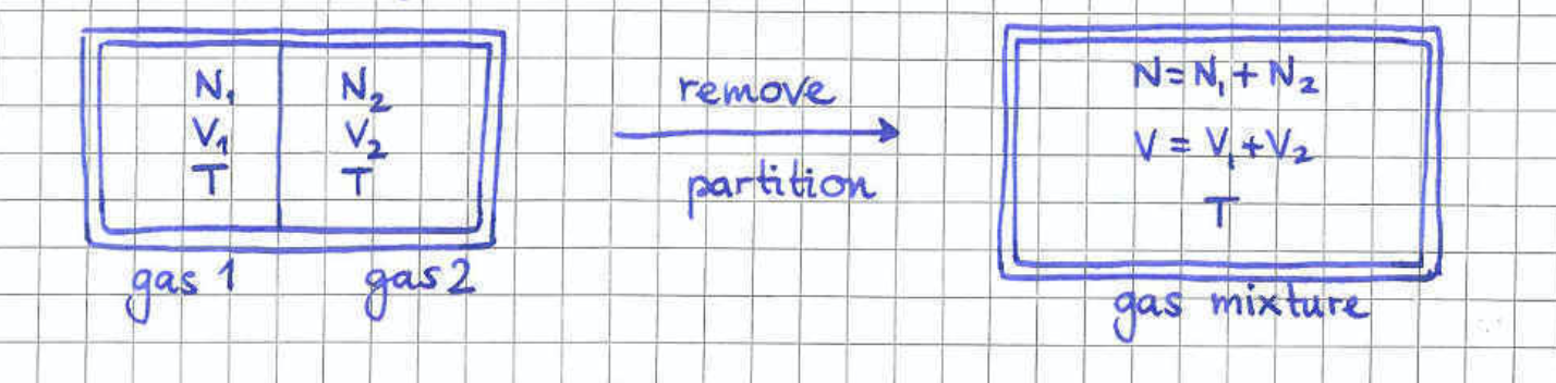
The fact that we find a non-extensive entropy even for such a simple system, is rather worrying but also very telling. It simply means that we have done something wrong at a very fundamental level. The deeper issue is more amplified when we consider the mixing of two gases. The scenario we have in mind is depicted in figure 4 where two gases which are held at the same pressure and temperature are initially separated by a wall. The wall is then removed resulting in the mixing of the two gases. In the following we will examine two different cases depending on whether the gas particles are identical or not.

Figure 4: Two systems of gases separated by a wall. The wall is then removed and the two gases mix with each other.

• The case of not identical gas particles

  For simplicity, we can assume that the particles of the two different gases have the same mass but different colour e.g. red for the left chamber and green for the right one. In this case, as soon we remove the wall the two gases will mix and there is no way we can bring the system to its original state. We wouldn’t be able to put the wall back and expect that all red particles will be on the left and all the red ones will be on the right. This is therefore an irreversible process and from basic thermodynamics the total entropy of the system has to increase. This implies that the mixing entropy

  $S_{mixing}=S_{fin}-S_{in}>0.$ (142)

  will be a strictly positive number. We see that the mixing of non-identical and therefore distinguishable particles would necessarily lead to positive mixing entropy.

• The case of identical gas particles

  We now examine the case where the two gases are composed of identical atoms. Since the two gases before mixing are at the same pressure and temperature , they will also have the same density $\rho =N_1/V_1=N_2/V_2$. This implies that after removing the wall, the mixture will retain the same density $\rho =(N_1+N_2)/(V_1+V_2)$. It is then obvious that if we put the wall back in its original position, the system will go back to its original thermodynamic state with two gases of particle numbers $N_1$ and $N_2$ inside volumes $V_1$ and $V_2$ held at temperature $T$. However, from the microscopic point of view, some of the particles which were original inside the left/right chamber have now relocated to the right/left chamber. From the point of view of classical mechanics this is a very different state from the original configuration. Nevertheless the above argument shows that the removal of the wall is a thermodynamically reversible process and therefore the mixing entropy should be zero.

  Let’s for a moment pretend that the expression (140) for the ideal gas entropy is correct. This allows us to compute the initial entropy

  $S_{in}$ $=S(\beta ,V_1,N_1)+S(\beta ,V_2,N_2)$

  $={\displaystyle \sum _{i=1}^2}{N}_i{k}_B\ln \left({\displaystyle \frac{V_i{e}^{\frac{3}{2}}}{{\lambda }^3}}\right),$ (143)

  and the final entropy

  $S_{fin}$ $=S(\beta ,V_1+V_2,N_1+N_2)$

  $=(N_1+N_2)\ln \left({\displaystyle \frac{(V_1+V_2)e^{\frac{3}{2}}}{{\lambda }^3}}\right).$ (144)

  The above yield the mixing entropy

  $S_{mixing}=-k_B\left(N_1\ln \left({\displaystyle \frac{N_1}{N_1+N_2}}\right)+N_2\ln \left({\displaystyle \frac{N_2}{N_1+N_2}}\right)\right)>0,$ (145)

  which can be easily seen to be a positive number, contrary to our expectation our thermodynamics argument. This is a good point to link this paradox to the non-extensivity of the entropy formula (140). The mixing entropy is,

  $S_{mixing}=S(\beta ,V_1+V_2,N_1+N_2)-S(\beta ,V_1,N_1)-S(\beta ,V_2,N_2),$ (146)

  which would be zero if $S(\beta ,V,N)$ was an extensive function of $V$ and $N$.

This mismatch between the Gibbs and the thermodynamic entropy is known as the Gibbs Paradox. Gibbs proposed that the paradox is resolved if classical microstates related by permutations of identical particles are treated as the same microstate. Therefore, identical classical particles should be treated as indistinguishable.

In more practical terms, whenever we need to count or sum over microstates, we can take all of the classically inequivalent microstates into account and then divide by $N!$, the number of permutations of $N$ objects. This is essentially the rule we wrote in equation (126). In the case of non-interacting identical particles then, for the $N$ particle partition function we can write,

$Z_N={\displaystyle \frac{1}{N!}}{Z}_1^N,$ (147)

where $Z_1$ is the single particle partition function. More generally, we have

$Z_N={\displaystyle \frac{1}{N!}}{\displaystyle {\int }_{{𝒫}_N}}{\displaystyle \prod _{i=1}^S}{\displaystyle \frac{d{q}_{i}d{p}_i}{h}}{e}^{-\beta H(q_i,p_i)},$ (148)

where $S$ is the total number of degrees of freedom in the system and ${𝒫}_N$ is the full classical phase space.

Here, we need to raise a point of caution about the validity of the ”$1/N!$” prescription. This works only for indistinguishable particles with a continuous set of microstates. To illustrate the issue, let’s consider a system of just two particles each of which is described by one position coordinate $q_i$ and its conjugate momentum $p_i$. The ”$1/N!$” prescription would correctly make configurations which have $(q_1,q_2,p_1,p_2)=(x_1,x_2,y_1,y_2)$ to configurations which have $(q_1,q_2,p_1,p_2)=(x_2,x_1,y_2,y_1)$. However, this division is not necessary for mictostates which have $q_1=q_2$ and $p_1=p_2$. The point here is that the configurations which are permutation invariant live on a hypersurface on ${𝒫}_2$ which doesn’t give a finite contribution to e.g. the partition function since it is a set of measure zero.

2.4 Non-interacting Indistinguishable Particles in the Grand Canonical Ensemble

In this section we will consider a system of non-interacting indistinguishable particles in the grand canonical ensemble where we keep $T$, $V$ and $\mu$ fixed. As we discussed in sections 1.2.2 and 1.2.3, the important quantities are the grand canonical partition function $𝒵(T,V,\mu )$ and the grand canonical potential $\mathrm{\Phi }$.

Since we don’t have any interactions between our indistinguishable particles, for the $N$-particle canonical partition function we can write

$Z(T,V,N)={\displaystyle \frac{1}{N!}}{Z}_1{(T,V)}^N,$ (149)

where $Z_1$ is the single particle partition function. Using this equation along with the relation (• ‣ 1.3) between the canonical and the grand canonical partition functions we obtain,

$𝒵(T,V,\mu )$ $={\displaystyle \sum _{N=0}^{\mathrm{\infty }}}{e}^{\beta \mu N}{\displaystyle \frac{1}{N!}}{Z}_1{(T,V)}^N$

$={\displaystyle \sum _{N=0}^{\mathrm{\infty }}}{\displaystyle \frac{1}{N!}}{\left(e^{\beta \mu }{Z}_1(T,V)\right)}^N$

$=e^{e^{\beta \mu }{Z}_1(T,V)}.$ (150)

According to equation (99), the grand canonical potential is,

$\mathrm{\Phi }(T,V,\mu )=-k_{B}T\ln 𝒵(T,V,\mu )=-{\displaystyle \frac{1}{\beta }}{e}^{\beta \mu }{Z}_1(T,V).$ (151)

We can now use the relation (1.2.4) to compute the average particle number,

$⟨N⟩=-{\displaystyle \frac{\partial \mathrm{\Phi }}{\partial \mu }}=e^{\beta \mu }{Z}_1(T,V).$ (152)

We now consider the thermodynamic limit $V\to \mathrm{\infty }$ where $⟨N⟩\to N$ to obtain an expression for the chemical potential in terms of the particle number, temperature and volume,

$\mu ={\displaystyle \frac{1}{\beta }}\ln \left({\displaystyle \frac{N}{Z_1(T,V)}}\right).$ (153)

The previous result is cute but we in order to learn something more about physics we are going to consider the case of the ideal gas. In that case the single particle partition function is given in equation (2.1) with the de Broglie wavelength defined as in (130). Combining these equations with our previous expression for the chemical potential we obtain,

$\mu ={\displaystyle \frac{1}{\beta }}\ln \left({\displaystyle \frac{N{\lambda }^3}{V}}\right).$ (154)

Equation (154) gives that the chemical potential is negative whenever . This coincides with the classical regime ${\lambda }^3\ll \frac{V}{N}$ where the de Broglie wavelength is much smaller than the length of the cubic space available to each particle. In the opposite case quantum effects would start becoming important and the classical description would break down.

At first sight, a negative chemical potential might sound counter intuitive sind the chemical potential is the change energy when adding a particle. However, this is meant to happen at fixed volume and entropy. The fact that the chemical potential is then negative suggests that we need to decrease the energy of the system in order for the entropy to remain unchanged after the increase in the particle number.

2.5 The Maxwell Distribution

The Maxwell distribution $P_M(v)$ gives the probability density for a gas atom to be found with speed $v$ when temperature and volume are kept fixed. In order to derive it for the ideal gas, we can start from the Boltzmann distribution of equation (20).

Suppose that we are interested in the speed probability distribution of the $j$-th particle in our system with position $\overrightarrow{q}\equiv {\overrightarrow{q}}_j$ and momentum $\overrightarrow{p}\equiv {\overrightarrow{p}}_j$. The first step is to obtain a probability density $p(\overrightarrow{p})$ for the momentum of that specific particle by integrating over the its position as well as the positions and momenta of the rest of the particles in the system. This procedure would give,

$p(\overrightarrow{p})={\displaystyle \frac{V{h}^{-3}}{Z_1}}{e}^{-\frac{\beta }{2m}{\overrightarrow{p}}^2},$ (155)

where the fact of $V$ comes from integrating over the coordinates of our particle. The extra factor of $h^{-}3$ comes from the fact that we are interested in a density which is supposed to be integrated over momenta. One can see that this is dimensionally sensible since $V{h}^{-3}$ has units of ${[\mathrm{momentum}]}^{-3}$. The next step is to obtain the probability density $P(\overrightarrow{v})$ for its velocity $\overrightarrow{v}$ by using the relation $\overrightarrow{p}=m\overrightarrow{v}$. Starting from the infinitesimal probability in momentum which we obtain by multiplying the probability density with the momentum space volume element we have,

$p(\overrightarrow{p})d^{3}p=m^{3}p(m\overrightarrow{v})d^{3}v=P(\overrightarrow{v})d^{3}v.$ (156)

From the above we can read off the relation,

$P(\overrightarrow{v})=m^{3}p(m\overrightarrow{v})={\displaystyle \frac{m^{3}V{h}^{-3}}{Z_1}}{e}^{-\frac{\beta m}{2}{\overrightarrow{v}}^2}.$ (157)

The final step is to use the velocity probability distribution $P(\overrightarrow{v})$ in order to derive the Maxwell distribution $P_M(v)$ which is a density in the velocity norm,

$v=\sqrt{v_x^2+v_y^2+v_z^2}.$ (158)

In order to do this, we move from the Cartesian coordinates $(v_x,v_y,v_y)$ to spherical ones $(v,\theta ,\varphi )$ parametrising the norm and the direction of $\overrightarrow{v}$ with and . Doing so we obtain the infinitesimal probabilities,

$P(v_x,v_y,v_z)d{v}_{x}d{v}_{y}d{v}_z=P(v)\sin \theta v^{2}dvd\theta d\varphi ,$ (159)

where we used the fact that $P(\overrightarrow{v})$ only depends on the norm of the velocity vector $\overrightarrow{v}$. The above shows that the Maxwell distribution we are after is,

$P_M(v)$ $={\displaystyle {\int }_0^{\pi }}\sin \theta d\theta {\displaystyle {\int }_0^{2\pi }}𝑑\varphi v^{2}P(v)$

$={\displaystyle \frac{4\pi m^{3}V{h}^{-3}}{Z_1}}{v}^2{e}^{-\frac{\beta m}{2}{v}^2}$

$=4\pi {\left({\displaystyle \frac{m}{2\pi k_{B}T}}\right)}^{\frac{3}{2}}{v}^2{e}^{-\frac{m}{2k_{B}T}{v}^2},$ (160)

which can be checked to be correctly normalised according to,

${\displaystyle {\int }_0^{\mathrm{\infty }}}𝑑v{P}_M(v)=1.$ (161)

Moreover, we can compute,

$⟨v^2⟩={\displaystyle {\int }_0^{\mathrm{\infty }}}𝑑v{v}^2{P}_M(v)={\displaystyle \frac{3k_{B}T}{m}},$ (162)

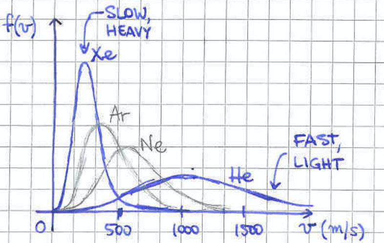
allowing us to compute the average energy $⟨E⟩=\frac{1}{2}m⟨v^2⟩=\frac{3}{2}{k}_{B}T$, agreeing with the results of section 2.2. As we can see, the average energy is solely fixed by the temperature, independently of the mass of the particle. This is compatible with the form of the distribution (2.5) which for fixed temperature suggests that heavier particles are more likely to have lower speed that heavier particles. Plotting the distribution (2.5) for different masses at a given temperature gives the picture of figure 5.

Figure 5: The Maxwell distribution for different masses, at a fixed temperature.

We have derived the Maxwell distribution from first principles, starting form the ideal gas. However, when Maxwell derived it didn’t know about statistical mechanics. He only relied on:

• Rotation symmetry

• Statistical independence of the velocity components $v_x$, $v_y$ and $v_z$

Rotational symmetry, or more precisely isotropy, implies that the probability density $\varphi (v_i)$ for each velocity component is given by the same function. Statistical independence implies then that the probability $dP$ to find the particle with velocity $\overrightarrow{v}$ in the parallelogram $[,v_x+d{v}_x]\times [v_y,v_y+d{v}_y]\times [v_z,v_z+d{v}_z]$ is

$dP=\varphi (v_x)\varphi (v_y)\varphi (v_z)d{v}_{x}d{v}_{y}d{v}_z.$ (163)

Going once again to spherical coordinates we should be able to write,

$dP=F(v)v^{2}dv\sin \theta d\theta d\varphi ,$ (164)

where $v$ is the norm of $\overrightarrow{v}$. Equating the two expressions above, and transforming the volume element we obtain the constraint,

$F(\sqrt{v_x^2+v_y^2+v_z^2})=\varphi (v_x)\varphi (v_y)\varphi (v_z).$ (165)

The above constraint can only be satisfied by a $\varphi$ of the form,

$\varphi (v_i)=A{e}^{-B{v}_i^2}.$ (166)

The velocity probability density is then given after integrating over the angular coordinates $\theta$ and $\varphi$ to obtain,

$P_M(v)=v^{2}F(v)=4\pi A^3{v}^2{e}^{-B{v}^2}.$ (167)

This expression has the same function dependence on $v$ with the function we derived in equation (2.5). We are left with two unknown constants which can be fixed by imposing the following two constraints,

• ${\int }_0^{\mathrm{\infty }}𝑑v{P}_M(v)=1$

• $⟨v^2⟩={\int }_0^{\mathrm{\infty }}𝑑v{v}^2{P}_M(v)=\frac{3k_{B}T}{m}$

2.6 The Diatomic Gas

In this subsection we will study a system of $N$ non-interacting diatomic molecules. This will let us see the importance of Quantum Mechanical effects in real world systems. More specifically, our aim is to compute the heat capacity of a diatomic gas as a function of temperature and compare it to experimental results. The resulting discrepancy has been one of the biggest puzzles of the 19th century. Here, we will use it to understand the limitations of the classical description of nature.

Since the system is non-interacting, we will focus on a single molecule in order to derive the single particle partition function. Our first step is to construct the Hamiltonian describing our molecule. A simple model for our molecule is based on the following assumptions:

• Two identical atoms of mass $m$ at positions ${\overrightarrow{x}}_1$ and ${\overrightarrow{x}}_2$ which are interconnected by a spring of natural length $2l$. The potential between the two particles is then $V=\frac{1}{4}m{\omega }^2{(|{\overrightarrow{x}}_2-{\overrightarrow{x}}_1|-2l)}^2$.

• The vibrations of the molecule are not too wild. In mathematical terms, the distance between the two atoms is very close to the natural length of the spring and $|{\overrightarrow{x}}_1-{\overrightarrow{x}}_2|\approx l$.

The above picture suggests that the degrees of freedom of a single molecule can be separated to translations of the whole molecule and rotations as well as vibrations which happen in the rest frame of the center of mass.

In full generality, the Lagrangian of the molecule is,

$L=T-V={\displaystyle \frac{1}{2}}m{\dot{\overrightarrow{x}}}_1^2+{\displaystyle \frac{1}{2}}m{\dot{\overrightarrow{x}}}_1^2-{\displaystyle \frac{1}{4}}m{\omega }^2{(|{\overrightarrow{x}}_2-{\overrightarrow{x}}_1|-2l)}^2.$ (168)

As is common in cases where the interaction potential has translational invariance, it is now useful to introduce the center mass $\overrightarrow{X}$ by changing variables according to,

${\overrightarrow{x}}_1$ $=\overrightarrow{X}+\overrightarrow{y},$

${\overrightarrow{x}}_2$ $=\overrightarrow{X}-\overrightarrow{y},$ (169)

and $\overrightarrow{y}$ is half of the vector pointing from one atom to the other. This leads to the Lagrangian

$L={\displaystyle \frac{M}{2}}{\dot{\overrightarrow{X}}}^2+{\displaystyle \frac{M}{2}}{\dot{\overrightarrow{y}}}^2-{\displaystyle \frac{1}{2}}M{\omega }^2{(|\overrightarrow{y}|-l)}^2,$ (170)

where $M=2m$ is the total mass of the molecule. The first term is really the Lagrangian of the center of mass which due to translational invariance behaves like a free particle of mass $M$. The second and the third terms govern the relative motion of the two atoms. We now want to separate the rotations from the vibrations by using spherical coordinates according to,

$y_x$ $=(l+\zeta )\sin \theta \cos \varphi ,$

$y_y$ $=(l+\zeta )\sin \theta \sin \varphi ,$

$y_z$ $=(l+\zeta )\cos \theta ,$ (171)

with and . This change of variables gives us the action

$L={\displaystyle \frac{M}{2}}{\dot{\overrightarrow{X}}}^2+{\displaystyle \frac{M{(l+\zeta )}^2}{2}}\left({\dot{\theta }}^2+{\sin }^2\theta {\dot{\varphi }}^2\right)+{\displaystyle \frac{M}{2}}{\dot{\zeta }}^2-{\displaystyle \frac{1}{2}}M{\omega }^2{\zeta }^2.$ (172)

This Lagrangian is still exact without having used the approximation of small vibrations. Moreover, we see that the rotational and vibrational degrees of freedom are coupled due to the factor ${(l+\zeta )}^2$ in front of the second term. This is precisely where the assumption of small vibrations is going to be useful. By setting $l+\zeta \approx l$ we are essentially decoupling those two degrees of freedom. After this assumption, the Lagrangian takes the form,

$L$ $=L_T+L_R+L_V,$

$L_T$ $={\displaystyle \frac{M}{2}}{\dot{\overrightarrow{X}}}^2,$

$L_R$ $={\displaystyle \frac{M{l}^2}{2}}\left({\dot{\theta }}^2+{\sin }^2\theta {\dot{\varphi }}^2\right),$

$L_V$ $={\displaystyle \frac{M}{2}}{\dot{\zeta }}^2-{\displaystyle \frac{1}{2}}M{\omega }^2{\zeta }^2.$ (173)

After this split, we can now derive the Hamiltonian of our molecule term by term with a very clean interpretation.

• $H_T$ for translations with respect to the $\overrightarrow{X}$ degrees of freedom

  The conjugate momentum is

  ${\overrightarrow{p}}_X={\displaystyle \frac{\partial L}{\partial \dot{\overrightarrow{X}}}}={\displaystyle \frac{\partial L_T}{\partial \dot{\overrightarrow{X}}}}=M\dot{\overrightarrow{X}},$ (174)

  yielding the Hamiltonian,

  $H_T=\dot{\overrightarrow{X}}\cdot {\overrightarrow{p}}_X-L_T={\displaystyle \frac{{\overrightarrow{p}}_X^2}{2M}}.$ (175)

• $H_R$ for rotations with respect to the $(\theta ,\varphi )$ degrees of freedom

  The conjugate momenta are,

  $p_{\theta }$ $={\displaystyle \frac{\partial L}{\partial \dot{\theta }}}={\displaystyle \frac{\partial L_R}{\partial \dot{\theta }}}=M{l}^2\dot{\theta },$

  $p_{\varphi }$ $={\displaystyle \frac{\partial L}{\partial \dot{\varphi }}}={\displaystyle \frac{\partial L_R}{\partial \dot{\varphi }}}=M{l}^2{\sin }^2\theta \dot{\varphi }.$ (176)

  The corresponding Hamiltonian is then,

  $H_R=\dot{\varphi }{p}_{\varphi }+\dot{\theta }{p}_{\theta }-L_R={\displaystyle \frac{1}{2I}}\left(p_{\theta }^2+{\displaystyle \frac{p_{\varphi }^2}{{\sin }^2\theta }}\right)$ (177)

  where we have defined the angular moment of inertia $I=M{l}^2$.

• $H_V$ for vibrations with respect to the $\zeta$ degree of freedom

  The conjugate momentum is,

  $p_{\zeta }={\displaystyle \frac{\partial L}{\partial \zeta }}={\displaystyle \frac{\partial L_V}{\partial \zeta }}=M\dot{\zeta }.$ (178)

  The corresponding Hamiltonian is then,

  $H_V=\dot{\zeta }{p}_{\zeta }-L_V={\displaystyle \frac{p_{\zeta }^2}{2M}}+{\displaystyle \frac{1}{2}}M{\omega }^2{\zeta }^2.$ (179)

After this derivation, the full Hamiltonian that we are going to need is,

$H=H_T(\overrightarrow{X},{\overrightarrow{p}}_X)+H_R(\theta ,\varphi ,p_{\theta },p_{\varphi })+H_V(\zeta ,p_{\zeta }).$ (180)

For the single particle partition function we can then write,

$Z_1(\beta ,V)=$ ${\displaystyle \frac{1}{h^6}}{\displaystyle \int d^{3}X{d}^3{p}_X𝑑\theta 𝑑p_{\theta }𝑑\varphi 𝑑p_{\varphi }𝑑\zeta 𝑑p_{\zeta }{e}^{-\beta H}}$

$=$ $\left({\displaystyle \int \frac{d^{3}X{d}^3{p}_X}{h^3}{e}^{-\beta H_T(\overrightarrow{X},{\overrightarrow{p}}_X)}}\right)\left({\displaystyle \int \frac{d\theta d{p}_{\theta }d\varphi d{p}_{\varphi }}{h^2}{e}^{-\beta H_R(\theta ,\varphi ,p_{\theta },p_{\varphi })}}\right)$

$\left({\displaystyle \int \frac{d\zeta d{p}_{\zeta }}{h}{e}^{-\beta H_V(\zeta ,p_{\zeta })}}\right)$

$=$ $Z_T(\beta ,V)Z_R(\beta ,V)Z_V(\beta ,V).$ (181)

In the last line we have decomposed the partition function into a translational, a rotational and a vibrational factor. Having in mind the heat capacity, our first step is compute the average energy of the $N$-body system whose partition function is

$Z_N=Z_1^N={(Z_T(\beta ,V)Z_R(\beta ,V)Z_V(\beta ,V))}^N.$ (182)

Using our formula (1.1.4) for the average energy of the canonical ensemble we have,

$⟨E⟩$ $=-{\displaystyle \frac{\partial }{\partial \beta }}\ln Z_N$

$=N\left(-{\displaystyle \frac{\partial }{\partial \beta }}\ln Z_T-{\displaystyle \frac{\partial }{\partial \beta }}\ln Z_R-{\displaystyle \frac{\partial }{\partial \beta }}\ln Z_V\right)$

$={⟨E⟩}_T+{⟨E⟩}_R+{⟨E⟩}_V.$ (183)

The above shows that the factorisation of the partition function in equation (2.6) sharpens the contribution of each degree of freedom to the average energy. Going back to our computation we can easily compute

$Z_T$ $={\displaystyle \int \frac{d^{3}X{d}^3{p}_X}{h^3}{e}^{-\beta \frac{{\overrightarrow{p}}_X^2}{2M}}}={\displaystyle \frac{V}{{\lambda }^3}},$

$Z_R$ $={\displaystyle \int \frac{d\theta d{p}_{\theta }d\varphi d{p}_{\varphi }}{h^2}{e}^{-\frac{\beta }{2I}\left(p_{\theta }^2+\frac{p_{\varphi }^2}{{\sin }^2\theta }\right)}}$

$={\displaystyle \frac{1}{h^2}}\sqrt{{\displaystyle \frac{2\pi I}{\beta }}}{\displaystyle {\int }_0^{\pi }}𝑑\theta \sqrt{{\displaystyle \frac{2\pi I{\sin }^2\theta }{\beta }}}{\displaystyle {\int }_0^{2\pi }}𝑑\varphi ={\displaystyle \frac{2I}{\beta {\mathrm{\hslash }}^2}}$

$Z_V$ $={\displaystyle \int \frac{d\zeta d{p}_{\zeta }}{h}{e}^{-\beta \left(\frac{p_{\zeta }^2}{2M}+\frac{1}{2}M{\omega }^2{\zeta }^2\right)}}={\displaystyle \frac{1}{\beta \mathrm{\hslash }\omega }},$ (184)

where the de Broglie wavelength $\lambda$ is as defined in equation (130). After this, the contributions of the individual degrees of freedom to the average energy are,

${⟨E⟩}_T$ $={\displaystyle \frac{3}{2}}N{k}_{B}T,$

${⟨E⟩}_R$ $=N{k}_{B}T,$

${⟨E⟩}_V$ $=N{k}_{B}T.$ (185)

Notice that we could had reached these conclusions about ${⟨E⟩}_T$ and ${⟨E⟩}_V$ solely from the equipartition theorem of subsection 2.2. After using the expression of equation (29), we obtain the corresponding heat capacity contributions

$C_T$ $={\displaystyle \frac{3}{2}}N{k}_B,$

$C_R$ $=N{k}_B,$

$C_V$ $=N{k}_B,$ (186)

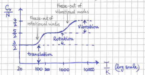
yielding the total heat capacity $C=\frac{7}{2}N{k}_B$. We see that all degrees of freedom contribute the same amount to the heat capacity, leading to a temperature independent constant. However, this result disagrees with the experimental data shown in figure 6. It is clear that as the temperature is lowered the different degrees of freedom freeze-out offering no contribution to the specific heat. This is purely a Quantum Mechanical effect, tied to the fact that the energy levels of a Quantum system are discreet.

Figure 6: The experimental curve for the heat capacity of a diatomic gas as a function of temperature. The rotational and vibrational degrees of freedom freeze as we lower the temperature.

To see the effect of freezing out for the vibrational degrees of freedom, it is useful to remember the specific heat in the example of the Quantum Mechanical simple harmonic oscillator of frequency $\omega$. The formula we derived in the corresponding homework problem was,

$C_V^{quant}=N{k}_B{\displaystyle \frac{{\left(\frac{\mathrm{\hslash }\omega }{2k_{B}T}\right)}^2}{{\sinh }^2\left(\frac{\mathrm{\hslash }\omega }{2k_{B}T}\right)}}.$ (187)

From this formula we see that the specific heat interpolates between $N{k}_B$ at $T\to \mathrm{\infty }$ down to zero as we take the limit $T\to 0$. The crossover between the two behaviours is when $k_{B}T\approx \mathrm{\hslash }\omega$. In more physics terms, this is when the typical thermal energy in the system $k_{B}T$ is approximately equal to the energy difference between the quantised energy levels of the system which go like $E_n=\mathrm{\hslash }\omega \left(n+\frac{1}{2}\right)$. Most importantly this is the energy gap between the ground state and the first excited state.

2.7 Weakly Interacting Gases - The Virial Expansion

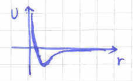
So far we have studied gases of non-interacting particles. In this subsection we will consider gases with non-zero interparticle interactions which are under control. A reasonable class of interactions to study vanish when the particles are too far away from each other and lead to repulsion when particles get too close. An example of such a potential is depicted in figure 7 where we can see that there is a characteristic distance $r_0$ above which the potential is very small. Two physically interesting potentials of this class are the Lenard-Jones potential

$V(r)=A{\left({\displaystyle \frac{r_0}{r}}\right)}^{12}-C{\left({\displaystyle \frac{r_0}{r}}\right)}^6,$ (188)

and the hard-core potential,

(189)

Figure 7: Example of potential exhibiting a strongly repulsive region at short distances and asymptotic freedom at infinity.

Given the above constraints, it is natural to guess that the effects of these interactions on the statistical behaviour of our gas is going to be controlled by the density $N/V$. Intuitively, we expect that the equation of state will have the leading behaviour of the ideal gas as in equation (135) and that it will receive corrections according to the Virial expansion,

${\displaystyle \frac{p}{k_{B}T}}={\displaystyle \frac{N}{V}}+B_2(T){\left({\displaystyle \frac{N}{V}}\right)}^2+B_3(T){\left({\displaystyle \frac{N}{V}}\right)}^3+\mathrm{\cdots }.$ (190)

The temperature dependent Virial coefficients $B_i(T)$ can be determined from first principles by following the Mayer cluster expansion. Here, we will only determine $B_2(T)$ in terms of the inter-particle potential $V(\overrightarrow{r})$.

The see how this works, we first write down a general Hamiltonian of $N$ identical interacting particles,

(191)

where we have defined $r_{jk}\equiv |\overrightarrow{r_j}-{\overrightarrow{r}}_k|$. Thinking of indistinguishable particles, the partition function in equation (148) is no longer factorisable due to interactions. However, after integrating over momenta it takes the form,

(192)

where $\lambda$ is the de Broglie wavelength (130). In the absence of interactions with $V=0$, the remaining integral over positions would give a factor $V^N$ and we would recover the ideal gas partition function of equation (132).

We need to find a good expansion scheme in order to approximate the remaining integral in the partition function. A naive guess would be to expand the exponential assuming a small value for the exponent. This would fail due to the fact that no matter how high a temperature we consider (small $\beta$), at small distances the potential would blow up. A highly non-obvious expansion comes after introducing the Mayer function,

$f(r)=e^{-\beta V(r)}-1,$ (193)

which is always bounded and vanishes at infinity. More precisely, given the generic properties of our potential we have ${lim}_{r\to 0^{+}}f(r)=-1$ and ${lim}_{r\to +\mathrm{\infty }}f(r)=0$. Moreover, above the characteristic scale $r_0$ above which our potential vanishes, the Mayer function is very small.

Before we go back to the computation of the integral in the partition function (192), it is useful to appreciate the benefit of introducing the Mayer function. A simple way to see this is by considering the integral,

${\displaystyle {\int }_V}{d}^{3}r{e}^{-\beta V(r)}={\displaystyle {\int }_V}{d}^{3}r(1+f(r))=V+{\displaystyle {\int }_V}{d}^{3}rf(r).$ (194)

In the above expression, the difficult integral has been split into two terms. The first one is equal to the volume $V$. However, since the Mayer is approximately zero for $r>r_0$, the second term will be of order $r_0^3\ll V$. And therefore $f(r)$ has effectively helped us expand a non-trivial integral to a large term and a suppressed one. Moreover, since $f(r)$ is approximately zero outside the volume $V$, we can approximate integrals of $f(r)$ over the volume $V$ by,

${\displaystyle {\int }_V}{d}^{3}rf(r)\approx {\displaystyle {\int }_{{ℝ}^3}}{d}^{3}rf(r).$ (195)

To carry out the integral in (192) we introduce the notation $f_{jk}=f(r_{jk})$ allowing us to write,

$Z(\beta ,V,N)$

(198)

The first term in the integrand will simply give $V^N$ after performing the integral over all particle positions. According to the discussion of the previous paragraph, each power of the Mayer function in the other terms will be lowering the powers of volume by one. At this point it is natural to guess that the second term will offer the second Virial coefficient in the expansion of equation (190) and so on. Therefore, for our purposes it is enough to consider the first couple of terms in the integrand.

After noting that the second term gives a sum of $N(N-1)/2\approx N^2/2$ equal terms we can write,

${\displaystyle \frac{N(N-1)}{2}}{V}^{N-2}{\displaystyle \int d^3{r}_1{d}^3{r}_{2}f(r_{12})}$

$=$ ${\displaystyle \frac{N(N-1)}{2}}{V}^{N-2}{\displaystyle {\int }_V}{d}^{3}R{\displaystyle {\int }_{{ℝ}^3}}{d}^{3}rf(r)$

$=$ ${\displaystyle \frac{N(N-1)}{2}}{V}^{N-1}{\displaystyle {\int }_{{ℝ}^3}}{d}^{3}rf(r)$

$\approx$ ${\displaystyle \frac{N^2}{2}}{V}^{N-1}{\displaystyle {\int }_{{ℝ}^3}}{d}^{3}rf(r),$ (199)

where in the second line we change variable of integration according to,

$\overrightarrow{R}={\displaystyle \frac{1}{2}}({\overrightarrow{r}}_1+{\overrightarrow{r}}_2),\overrightarrow{r}={\overrightarrow{r}}_2-{\overrightarrow{r}}_1.$

Putting everything together, we have that

$Z(\beta ,V,N)$ $={\displaystyle \frac{1}{N!}}{\displaystyle \frac{V^N}{{\lambda }^{3N}}}\left(1+{\displaystyle \frac{N^2}{2V}}{\displaystyle {\int }_{{ℝ}^3}}{d}^{3}rf(r)+\mathrm{\cdots }\right)$

$\approx {\displaystyle \frac{1}{N!}}{\displaystyle \frac{V^N}{{\lambda }^{3N}}}{\left(1+{\displaystyle \frac{N}{2V}}{\displaystyle {\int }_{{ℝ}^3}}{d}^{3}rf(r)+\mathrm{\cdots }\right)}^N$

$=Z_{ideal}{\left(1+{\displaystyle \frac{N}{2V}}{\displaystyle {\int }_{{ℝ}^3}}{d}^{3}rf(r)+\mathrm{\cdots }\right)}^N,$ (200)

where we recognised the partition function of the ideal gas of equation (132) for $d=3$.

Since we want to compute the pressure of our gas, it is useful to compute the free energy. According to equation (1.1.8) this is given by,

$F$ $=-k_{B}T\ln Z(\beta ,B,N)$

$=-k_{B}T\ln Z_{ideal}-N{k}_{B}T\ln \left(1+{\displaystyle \frac{N}{2V}}{\displaystyle {\int }_{{ℝ}^3}}{d}^{3}rf(r)+\mathrm{\cdots }\right)$

$\approx F_{ideal}-N{k}_{B}T{\displaystyle \frac{N}{2V}}{\displaystyle {\int }_{{ℝ}^3}}{d}^{3}rf(r).$ (201)

We can now evaluate the pressure by using equation (70),

$p$ $=-{\displaystyle \frac{\partial F}{\partial V}}=-{\displaystyle \frac{\partial F_{ideal}}{\partial V}}-{\displaystyle \frac{1}{2}}{k}_{B}T{\left({\displaystyle \frac{N}{V}}\right)}^2{\displaystyle {\int }_{{ℝ}^3}}{d}^{3}rf(r)$

$=k_{B}T{\displaystyle \frac{N}{V}}-{\displaystyle \frac{1}{2}}{k}_{B}T{\left({\displaystyle \frac{N}{V}}\right)}^2{\displaystyle {\int }_{{ℝ}^3}}{d}^{3}rf(r)\Rightarrow$

${\displaystyle \frac{p}{k_{B}T}}$ $={\displaystyle \frac{N}{V}}+\left(-{\displaystyle \frac{1}{2}}{\displaystyle {\int }_{{ℝ}^3}}{d}^{3}rf(r)\right){\left({\displaystyle \frac{N}{V}}\right)}^2.$ (202)

Comparing the above expression with the Virial expansion (190) we can read off the second Virial coefficient,

$B_2(T)=-{\displaystyle \frac{1}{2}}{\displaystyle {\int }_{{ℝ}^3}}{d}^{3}rf(r).$ (203)

The above gives us an expression in terms of the potential $V(r)$ and the temperature $T$.

As an example, we will apply formula (203) for the case of the hard-core potential in equation (189). For this case, the Mayer function we need to integrate is,

(204)

After introducing spherical coordinates and integrating over the angular directions we obtain,

$B_2(T)$ $=-2\pi \left[-{\displaystyle {\int }_0^{r_0}}𝑑r{r}^2+{\displaystyle {\int }_{r_0}^{\mathrm{\infty }}}𝑑r{r}^2\left(e^{\beta V_0{\left(\frac{r_0}{r}\right)}^6}-1\right)\right]$

$=-2\pi \left[-{\displaystyle \frac{r_0^3}{3}}+{\displaystyle {\int }_{r_0}^{\mathrm{\infty }}}𝑑r{r}^2\left(e^{\beta V_0{\left(\frac{r_0}{r}\right)}^6}-1\right)\right].$ (205)

We see that the second integral, coming from the region of attraction, is still quite non-trivial in case we want to obtain a closed form for it. However, since the integrand is bounded in the whole region, we can consider the high temperature limit $\beta V_0\ll 1$. In this limit, we can expand the exponential at any value of $r$ to obtain,

$B_2(T)$ $=-2\pi \left[-{\displaystyle \frac{r_0^3}{3}}+{\displaystyle \frac{V_0{r}_0^6}{k_{B}T}}{\displaystyle {\int }_{r_0}^{\mathrm{\infty }}}𝑑r{r}^{-4}\right]$

$=-2\pi \left[-{\displaystyle \frac{r_0^3}{3}}+{\displaystyle \frac{V_0{r}_0^3}{3k_{B}T}}\right]$

$=b-{\displaystyle \frac{a}{k_{B}T}},$ (206)

where we have defined $a=\frac{2\pi r_0^3{V}_0}{3}$ and $b=\frac{2\pi r_0^3}{3}$. At this point it is useful to point out that $b$ comes from the repulsive region of the potential while $a$ represents the attractive.

Putting everything together with equation (190), the hard-core potential leads to the equation of state

${\displaystyle \frac{p}{k_{B}T}}={\displaystyle \frac{N}{V}}+\left(b-{\displaystyle \frac{a}{k_{B}T}}\right){\left({\displaystyle \frac{N}{V}}\right)}^2.$ (207)

This is our final answer but it is instructive to bring the equation of state in a slightly different form, the Van der Waals equation of state for an interacting gas. We have,

$\left(p+a{\displaystyle \frac{N^2}{V^2}}\right){\left(1+b{\displaystyle \frac{N}{V}}\right)}^{-1}$ $={\displaystyle \frac{N{k}_{B}T}{V}}\Rightarrow$

$\left(p+a{\displaystyle \frac{N^2}{V^2}}\right)\left(1-b{\displaystyle \frac{N}{V}}\right)$ $={\displaystyle \frac{N{k}_{B}T}{V}}\Rightarrow \Rightarrow$

$p$ $={\displaystyle \frac{N{k}_{B}T}{V-Nb}}-a{\displaystyle \frac{N^2}{V^2}},$ (208)

where in the second line we used the fact that $N/V$ is a small number in order to approximate,

${\left(1+b{\displaystyle \frac{N}{V}}\right)}^{-1}\approx 1-b{\displaystyle \frac{N}{V}}.$ (209)

It is now interesting to compare the Van der Waals equation (2.7) to the equation of state of the ideal gas,

$p^{\prime }={\displaystyle \frac{N{k}_{B}T}{V^{\prime }}}.$ (210)

It looks as if we have effectively replaced the volume $V^{\prime }$ by $V-Nb$ which is the volume available for a particle to explore due to the repulsion from the other particles. Moreover, the attractive part of the potential results in a reduction of the pressure, given by the term in (2.7) which is proportional to $a$.

Figure 8: The isotherms of the Van der Vaals equation (2.7).

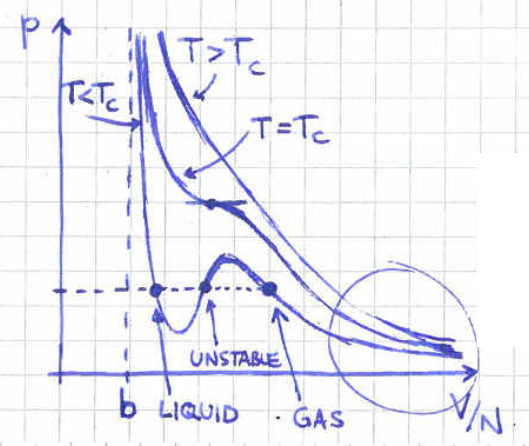
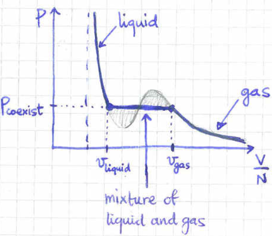
As an aside that the 4H students will study in more detail, another interesting feature of the Van der Waals equation of state (2.7) is the fact that it can capture a phase transition. To see this, in figure 8 we plot different isotherms in the $p-V$ diagram of equation (2.7). The diagram shows that there is a certain critical temperature $T_c=\frac{8}{27}\frac{a}{k_{B}b}$ below which the isotherms have three possible values of volume at fixed pressure.

The middle point $V_2$ is thermodynamically unstable since in that region the pressure seems to decrease as we decrease the volume. The volume $V_1$ represents the liquid phase while the volume $V_3$ represents the gas phase of our system. So, which point is the correct one? The answer is that the whole segment of the isotherm between the volumes $V_1$ and $V_2$ needs to be replaced by a flat line, as in figure LABEL:vdw2. The point of equilibrium between the liquid and the gas phase is determined by the Maxwell construction.

Figure 9: The correct isotherms connecting the liquid and gas phases of Van der Waals isotherms.

3 Quantum Gases

In the previous (especially in section 2.6), we came to appreciate that the discreteness of the energy levels in quantum Mechanics leads to a drastic change of thermodynamic systems at low temperatures. This is one consequence which is of course already there even in single particle systems. It was certainly interesting how this is propagated in the collective behaviour of large scale systems.

The first aim of this section is to provide a proof of how one can arrive at the classical partition function (21) after taking an appropriate limit of the quantum partition function (8). As we have mentioned before, the constant $h$ that appears in (21) was introduced by hand in order to make the partition function dimensionless. Here we will see how this constant naturally emerges from the classical limit of (8) and this is going to be identified with Planck’s constant which is secretly hiding in the energy levels $E_n$ of the quantum system.

The second aim of this section is to highlight even more striking quantum effects related to the very nature of quantum many body systems. In the previous sections, as far as many body systems are concerned, quantum mechanical particles were treated on equal footing with classical ones with the only difference being the discreteness of their energy levels. The aim of this section is to provide a more precise treatment of identical particles from the point of view of quantum Mechanics. As we will see, depending on how we can populate the energy levels in a many body system, quantum particles are divided into two large categories, the Bosons and the Fermions. As we will see, at high temperatures non-interacting gases of Bosons or Fermions look very similar to the classical ideal gas of section 2.1. However, at low temperatures they form two very different states of matter.

3.1 From Quantum to Classical

This section is for your own education since it assumes previous knowledge of quantum mechanics. In order to keep the discussion as simple as possible we will focus more on the single particle partition function in one spatial dimension. This is enough to illustrate the basic concepts and especially to show how the quantum mechanical origin of the factor$h^{-1}$ in the classical partition function (21).

The basic ingredients in our derivation will the the three eigenbasis $\left\{\mid x⟩\right\}$, $\mid p⟩$, $\mid n⟩$ corresponding to the position operator $\widehat{x}$, the momentum operator $\widehat{p}$ and the Hamiltonian $\widehat{H}$. As we know, these have to satisfy the eigenvalue problem equation,

$\widehat{x}\mid x⟩$ $=x\mid x⟩,x\in ℝ,$

$\widehat{p}\mid p⟩$ $=p\mid p⟩,p\in ℝ,$

$\widehat{H}\mid n⟩$ $=E_n\mid n⟩,n\in \mathbb{N}.$ (211)

At this point it is useful to remember the normalisation conventions,

$⟨x|x^{\prime }⟩=\delta (x-x^{\prime }),⟨p|p^{\prime }⟩=\delta (p-p^{\prime }),⟨n|n^{\prime }⟩={\delta }_{n,n^{\prime }},$ (212)

according to which eigenvectors corresponding to continuous spectra are normalised with Dirac’s delta while eigenvectors of discreet spectra are normalised with Kronecker’s delta. Moreover, we will find useful the inner product,

$⟨x|p⟩={\displaystyle \frac{1}{\sqrt{2\pi \mathrm{\hslash }}}}{e}^{\frac{i}{\mathrm{\hslash }}px},$ (213)

which can be derived from defining equation of the momentum operator

$⟨x\mid \widehat{p}\mid \psi ⟩=-i\mathrm{\hslash }{\displaystyle \frac{d}{dx}}⟨x|\psi ⟩.$ (214)

Since these are eigenbasis of Hermitian operators, we know that they must be complete. Given the normalisation of equation (212) we have three independent completeness relations,

$\widehat{𝕀}={\displaystyle {\int }_{-\mathrm{\infty }}^{+\mathrm{\infty }}}𝑑x\mid x⟩⟨x\mid ={\displaystyle {\int }_{-\mathrm{\infty }}^{+\mathrm{\infty }}}𝑑x\mid p⟩⟨p\mid ={\displaystyle \sum _{\mid n⟩}}\mid n⟩⟨n\mid ,$ (215)

where $\widehat{𝕀}$ is the identity operator in our Hilbert space.

Given a particular discreet orthonormal basis $\mid i⟩$, it is useful to define the trace of an operator $\widehat{A}$ according to,

$Tr(\widehat{A})={\displaystyle \sum _i}⟨i\mid \widehat{A}\mid i⟩.$ (216)

For a continuous basis $\mid q⟩$ we trace would be,

$Tr(\widehat{A})={\displaystyle \int 𝑑q⟨q\mid \widehat{A}\mid q⟩}.$ (217)

An important fact that our derivation will use is the fact that the trace is basis independent. Indeed, we can use the completeness relations (215) along with the orthogonality conditions (212) to show that e.g.

$Tr(\widehat{A})$ $={\displaystyle \sum _n}⟨n\mid \widehat{A}\mid n⟩={\displaystyle \sum _n}⟨n\mid \widehat{𝕀}\widehat{A}\widehat{𝕀}\mid n⟩$

$={\displaystyle {\int }_{-\mathrm{\infty }}^{+\mathrm{\infty }}}𝑑x{\displaystyle {\int }_{-\mathrm{\infty }}^{+\mathrm{\infty }}}𝑑x^{\prime }{\displaystyle \sum _{\mid n⟩}}⟨n|x⟩⟨x\mid \widehat{A}\mid x^{\prime }⟩⟨x^{\prime }|n⟩$

$={\displaystyle {\int }_{-\mathrm{\infty }}^{+\mathrm{\infty }}}𝑑x{\displaystyle {\int }_{-\mathrm{\infty }}^{+\mathrm{\infty }}}𝑑x^{\prime }\left({\displaystyle \sum _{\mid n⟩}}⟨x^{\prime }|n⟩⟨n|x⟩\right)⟨x\mid \widehat{A}\mid x^{\prime }⟩$

$={\displaystyle {\int }_{-\mathrm{\infty }}^{+\mathrm{\infty }}}𝑑x{\displaystyle {\int }_{-\mathrm{\infty }}^{+\mathrm{\infty }}}𝑑x^{\prime }⟨x^{\prime }\mid \left({\displaystyle \sum _{\mid n⟩}}\mid n⟩⟨n\mid \right)\mid x⟩⟨x\mid \widehat{A}\mid x^{\prime }⟩$

$={\displaystyle {\int }_{-\mathrm{\infty }}^{+\mathrm{\infty }}}𝑑x{\displaystyle {\int }_{-\mathrm{\infty }}^{+\mathrm{\infty }}}𝑑x^{\prime }⟨x^{\prime }\mid \widehat{𝕀}\mid x⟩⟨x\mid \widehat{A}\mid x^{\prime }⟩$

$={\displaystyle {\int }_{-\mathrm{\infty }}^{+\mathrm{\infty }}}𝑑x{\displaystyle {\int }_{-\mathrm{\infty }}^{+\mathrm{\infty }}}𝑑x^{\prime }\delta (x-x^{\prime })⟨x\mid \widehat{A}\mid x^{\prime }⟩$

$={\displaystyle {\int }_{-\mathrm{\infty }}^{+\mathrm{\infty }}}𝑑x⟨x\mid \widehat{A}\mid x⟩.$ (218)

In the second and fifth lines we used twice the completeness relation (215) and in the penultimate line the normalisation (212) yielded Dirac’s delta.

We now define the thermal density matrix ${\widehat{\rho }}_T=e^{-\beta \widehat{H}}$ which helps us write the quantum partition function (8) as a trace,

$Tr({\widehat{\rho }}_T)$ $={\displaystyle \sum _{\mid n⟩}}⟨n\mid e^{-\beta \widehat{H}}\mid n⟩={\displaystyle \sum _{\mid n⟩}}⟨n\mid e^{-\beta E_n}\mid n⟩$

$={\displaystyle \sum _{\mid n⟩}}{e}^{-\beta E_n}⟨n|n⟩={\displaystyle \sum _{\mid n⟩}}{e}^{-\beta E_n}=Z.$ (219)

In the above derivation we used that $e^{-\beta \widehat{H}}\mid n⟩=e^{-\beta E_n}\mid n⟩$ since $\mid n⟩$ is an eigenvector of $\widehat{H}$ with eigenvalue $E_n$. The independence of the basis now lets us write the trace in terms of the coordinate basis,

$Z={\displaystyle {\int }_{-\mathrm{\infty }}^{+\mathrm{\infty }}}𝑑x⟨x\mid e^{-\beta \widehat{H}}\mid x⟩.$ (220)

We are interested in the Hamiltonian of a particle moving inside a potential $V(x)$ which allows us to write the quantum mechanical Hamiltonian,

$\widehat{H}={\displaystyle \frac{1}{2m}}{\widehat{p}}^2+\widehat{V}(\widehat{x}).$ (221)

Since $\mid x⟩$ is an eigenvector of $\widehat{x}$ we know that $e^{-\beta \widehat{V}(\widehat{x})}\mid x⟩=e^{-\beta V(x)}\mid x⟩$. It is therefore very tempting to write the thermal density matrix that appears in the integrand of equation (220) as the product of $e^{-\frac{\beta }{2m}{\widehat{p}}^2}$ and $e^{-\beta \widehat{V}(\widehat{x})}$. Of course, we know that we cannot do this since ${\widehat{p}}^2$ and $\widehat{V}(\widehat{x})$ do not commute. In order to achieve something like this we would have to use the Zassenhaus identity,

$e^{\widehat{A}+\widehat{B}}=e^{\widehat{A}}{e}^{\widehat{B}}{e}^{-\frac{1}{2!}[\widehat{A},\widehat{B}]}{e}^{\frac{1}{3!}\left(2[\widehat{B},[\widehat{B},\widehat{A}]]+[\widehat{A},[\widehat{A},\widehat{B}]]\right)}\mathrm{\cdots },$ (222)

with the dots hiding higher order commutators between $\widehat{A}$ and $\widehat{B}$. In our case we have $\widehat{A}=-\frac{\beta }{2m}{\widehat{p}}^2$ and $\widehat{B}=-\beta \widehat{V}(\widehat{x})$. However, we know that every commutator of $\widehat{p}$ with $\widehat{x}$ would produce a factor of $\mathrm{\hslash }$ which we will take to be small in the classical approximation. Since we are interested in the classical limit, it is perfectly fine to approximate

$e^{-\beta \widehat{H}}\approx e^{-\frac{\beta }{2m}{\widehat{p}}^2}{e}^{-\beta \widehat{V}(\widehat{x})}+𝒪(\mathrm{\hslash }).$ (223)

This allow us to approximate the partition function in (220) according to,

$Z$ $\approx {\displaystyle {\int }_{-\mathrm{\infty }}^{+\mathrm{\infty }}}𝑑x⟨x\mid e^{-\frac{\beta }{2m}{\widehat{p}}^2}{e}^{-\beta \widehat{V}(\widehat{x})}\mid x⟩+𝒪(\mathrm{\hslash })$

$={\displaystyle {\int }_{-\mathrm{\infty }}^{+\mathrm{\infty }}}𝑑x⟨x\mid e^{-\frac{\beta }{2m}{\widehat{p}}^2}\mid x⟩e^{-\beta V(x)}+𝒪(\mathrm{\hslash })$

$={\displaystyle {\int }_{-\mathrm{\infty }}^{+\mathrm{\infty }}}𝑑x⟨x\mid e^{-\frac{\beta }{2m}{\widehat{p}}^2}\widehat{𝕀}\mid x⟩e^{-\beta V(x)}+𝒪(\mathrm{\hslash })$

$={\displaystyle {\int }_{-\mathrm{\infty }}^{+\mathrm{\infty }}}𝑑x{\displaystyle {\int }_{-\mathrm{\infty }}^{+\mathrm{\infty }}}𝑑p⟨x\mid e^{-\frac{\beta }{2m}{\widehat{p}}^2}\mid p⟩⟨p|x⟩e^{-\beta V(x)}+𝒪(\mathrm{\hslash })$

$={\displaystyle {\int }_{-\mathrm{\infty }}^{+\mathrm{\infty }}}𝑑x{\displaystyle {\int }_{-\mathrm{\infty }}^{+\mathrm{\infty }}}𝑑p⟨x|p⟩⟨p|x⟩e^{-\frac{\beta }{2m}{p}^2}{e}^{-\beta V(x)}+𝒪(\mathrm{\hslash })$

$={\displaystyle {\int }_{-\mathrm{\infty }}^{+\mathrm{\infty }}}𝑑x{\displaystyle {\int }_{-\mathrm{\infty }}^{+\mathrm{\infty }}}𝑑p⟨x|p⟩⟨p|x⟩e^{-\beta H(x,p)}+𝒪(\mathrm{\hslash })$

$={\displaystyle {\int }_{-\mathrm{\infty }}^{+\mathrm{\infty }}}𝑑x{\displaystyle {\int }_{-\mathrm{\infty }}^{+\mathrm{\infty }}}𝑑p{\displaystyle \frac{1}{2\pi \mathrm{\hslash }}}{e}^{-\beta H(x,p)}+𝒪(\mathrm{\hslash })$

$={\displaystyle \int \frac{dxdp}{h}{e}^{-\beta H(x,p)}}+𝒪(\mathrm{\hslash }).$ (224)

In the last line we see that the leading term in an $\mathrm{\hslash }$-expansion is the classical single particle partition function with the correct factor of $h^{-1}$! It is probably good to give some comments about the various steps in the above derivation. In the fourth line we used the completeness relation (215) in terms of the momentum eigenvectors which allowed us to exploit the fact that $e^{-\frac{\beta }{2m}{\widehat{p}}^2}\mid p⟩=e^{-\frac{\beta }{2m}{p}^2}\mid p⟩$ in the line below. In the penultimate line we simply used that inner result of equation (213) for the inner product of $\widehat{x}$ with $\widehat{p}$.

3.2 Single Particle in a Box

This subsection is a prelude before we consider non-interacting gases of Bosons and Fermions. The aim is to come up with a precise description of the single particle microstates of a particle inside a box of side $L$.

To set up the problem of finding the microstates, we need to solve the eigenvalue problem,

$\widehat{H}{\psi }_n(x,y,z)=E_n{\psi }_n(x,y,z),$ (225)

with periodic boundary conditions on the sides of the box,

${\psi }_n(x,y,z)={\psi }_n(x+L,y,z)={\psi }_n(x,y+L,z)={\psi }_n(x,y,z+L).$ (226)

A more natural set of boundary conditions would be that the wavefunction vanishes on the sides of the box but the physics will remain unchanged.

According the the general rules of Quantisation of classical systems, the Hamiltonian of the free particle can be found by replacing the classical momentum $p_i$ according to,

$p_i\to -i\mathrm{\hslash }{\partial }_i.$ (227)

This suggests that for a non-relativistic particle we would have

$\widehat{H}=-{\displaystyle \frac{{\mathrm{\hslash }}^2}{2m}}{\nabla }^2.$ (228)

An effective Hamiltonian we can write down for a relativistic particle is,

$\widehat{H}=\sqrt{-c^2{\mathrm{\hslash }}^2{\nabla }^2+m^2{c}^4}.$ (229)

In both cases, we see that the Hamiltonian is function of the Laplace operator ${\nabla }^2$. It is therefore easy to see that the wavefunctions that solve the eigenvalue problem equation (3.1) are of the form

${\psi }_{\overrightarrow{k}}(\overrightarrow{x})={\displaystyle \frac{1}{L^{3/2}}}{e}^{i\overrightarrow{k}\cdot \overrightarrow{x}},$ (230)

for an arbitrary vector $\overrightarrow{k}$ and we have included an appropriate normalisation factor for our wavefunction so that,

${\displaystyle {\int }_V}{d}^{3}x{\psi }_{\overrightarrow{k}}^{\ast }(\overrightarrow{x}){\psi }_{\overrightarrow{k}}(\overrightarrow{x})=1.$ (231)

Plugging the eigenfunction (230) in the eigenvalue problem equation (3.1) we can extract the eigenvalue for the energy in terms of the vector $\overrightarrow{k}$. For the non-relativistic particle with Hamiltonian (228) we have

$E(\overrightarrow{k})=E(k)={\displaystyle \frac{{\mathrm{\hslash }}^2{k}^2}{2m}},$ (232)

where $k=\sqrt{{\overrightarrow{k}}^2}$ is the modulus of the wave-vector. For the relativistic particle with Hamiltonian (229) we have,

$E(k)=\sqrt{c^2{\mathrm{\hslash }}^2{k}^2+m^2{c}^4}.$ (233)

So far, we haven’t implemented the boundary conditions (226) of our problem. Using the wavefunction (230), we see that this implies a quantisation condition for the wavevector,

${\overrightarrow{k}}_{\overrightarrow{n}}={\displaystyle \frac{2\pi }{L}}\overrightarrow{n},\overrightarrow{n}\in {\mathbb{Z}}^3.$ (234)

We therefore see that the microstates of a free particle inside a box are parametrised by three integers $n_i$ and the corresponding energy levels given by (232) and (233) are discreet as we would expect for a quantum system in a finite volume.

To summarise the important results of this subsection:

• The energy levels are given by a function $E(k)$ of the modulus of the wavevector $\overrightarrow{k}$. For the non-relativistic particle we have equation (232) while for the relativistic we have (233).

• The single particle quantum states are labelled by three integers $n_i$ with the discreet wavevector given by (234). The corresponding discreet energy levels are given by $E_{\overrightarrow{n}}=E(k_{\overrightarrow{n}})$.

3.2.1 Density of Single Particle States

Another important quantity we would like to study is the density of states $g(E)$ for a single free particle moving inside a macroscopic box. The density of states for a Quantum System was first introduced in equation (116) of section 1.3. Here, we will approximate the function (116) in the case of a particle moving inside a box whose side $L$ is much greater that the de Broglie wavelength (130) of the particle. To appreciate this last point we point out the single particle partition function

$Z_1$ $={\displaystyle \sum _{n_x,n_y,n_z}}{e}^{-\beta E_{\overrightarrow{n}}}={\displaystyle \sum _{n_x,n_y,n_z}}{e}^{-\frac{2\beta {\mathrm{\hslash }}^2{\pi }^2}{m{L}^2}(n_x^2+n_y^2+n_z^2)}$

$={\displaystyle \sum _{n_x,n_y,n_z}}{e}^{-\frac{{\lambda }^2}{L^2}(n_x^2+n_y^2+n_z^2)}.$ (235)

By simply staring at the dimensionless exponent, we see that we are indeed comparing the de Broglie wavelength $\lambda$ to the macroscopic lengthscale $L$ of our container.

One way to find the density of states is by simply using the definition (116). For the single particle in a box that would simply be,

$g(E)={\displaystyle \sum _{\overrightarrow{n}}}\delta (E-E(k_{\overrightarrow{n}})).$ (236)

However, we are going to take a slightly different approach. We will remember that the density of density is designed so that for any function of energy $f(E)$ which we are summing over all microstates we can write,

$I={\displaystyle \sum _{\overrightarrow{n}}}f(E(k_{\overrightarrow{n}}))={\displaystyle \int 𝑑Eg(E)f(E)}.$ (237)

In order to approximate the energy density of states, we imagine that we need to perform a sum whose terms depend only on the energy levels,

$I$ $={\displaystyle \sum _{\overrightarrow{n}}}f(E(k_{\overrightarrow{n}}))={\displaystyle \sum _{{\overrightarrow{k}}_{\overrightarrow{n}}}}f(E(k_{\overrightarrow{n}}))$

$={\displaystyle \frac{V}{{(2\pi )}^3}}{\displaystyle \sum _{{\overrightarrow{k}}_{\overrightarrow{n}}}}{(\mathrm{\Delta }k)}^{3}f(E(k_{\overrightarrow{n}})),$ (238)

where we introduced the spacing $\mathrm{\Delta }k=\frac{2\pi }{L}$ of the quantisation condition in equation (234) and the volume $V=L^3$. In the large volume limit we see that $\mathrm{\Delta }k\to 0$ and we can approximate the sum by an integral in three dimensions,

$I$ $\to {\displaystyle \frac{V}{{(2\pi )}^3}}{\displaystyle {\int }_{{ℝ}^3}}{d}^{3}kf(E(k))$

$={\displaystyle \frac{V}{{(2\pi )}^3}}\mathrm{\hspace{0.17em}4}\pi {\displaystyle \int 𝑑k{k}^{2}f(E(k))},$ (239)

where in the second line we exploited the fact that energy only depends on the modulus of the wavevector and we introduced spherical coordinates. Integrating over the angular directions yielded a factor of $4\pi$. In order to read off the density of states, we will now trade the modulus of the wavevector for the energy by inverting the dispersion relation $E=E(k)$ to write $k=k(E)$. Our integral then becomes,

$I={\displaystyle \frac{V}{{(2\pi )}^3}}\mathrm{\hspace{0.17em}4}\pi {\displaystyle \int 𝑑E\frac{d}{dE}k(E)k^2(E)f(E)}.$ (240)

This suggests that, according to the alternative definition of equation (237), in our approximation the density of states is

$g(E)={\displaystyle \frac{V}{2{\pi }^2}}{\displaystyle \frac{d}{dE}}k(E)k^2(E),$ (241)

allowing us to write,

$Q={\displaystyle \int 𝑑Eg(E)f(E)}.$ (242)

Of particular interest to us is going to be the non-relativistic particle. Inverting its dispersion relation (232) gives $k=\frac{\sqrt{2mE}}{\mathrm{\hslash }}$ which we can use in (241) to obtain the density of states,

$g(E)={\displaystyle \frac{V}{4{\pi }^2}}{\left({\displaystyle \frac{2m}{{\mathrm{\hslash }}^2}}\right)}^{\frac{3}{2}}{E}^{1/2}.$ (243)

Applying the same logic for the relativistic particle and its dispersion relation (233) we obtain the density of states,

(244)

3.3 Bosons vs Fermions

Apart from their mass and electric charge, elementary particles are characterised by an additional number, the spin $s$ which is a purely quantum mechanical property. Bosons have integer spin while Fermions have a half-integer spin.

The Higgs field is a spin zero particle while examples of spin $1/2$ particles are the electron, the quarks and the neutrinos. Spin $1$ particles include the photon which is responsible for the electromagnetic interaction and the gluons which carry the strong nuclear force of QCD. There are no known spin $3/2$ elementary particles while the graviton which is the particle that mediates the gravitational force has spin equal to $2$.

From the point of view of statistical physics, Bosons and Fermions follow very different rules. From a more fundamental point of view, this is a consequence of the Spin-Statistics which requires the techniques of Quantum Field Theory. From the point of view of quantum mechanics it simply states that when exchanging two:

• Fermions, the quantum state vector is antisymmetric

• Bosons, the quantum state vector is symmetric

Reading these statements slightly differently we can say that,

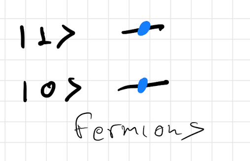
• Two identical Fermions cannot occupy the same single particle microstate

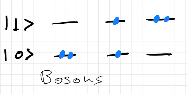
• Two or more identical Bosons can occupy the same single particle microstate

To summarise what we have seen so far in this course we can have three different kinds of identical particles:

• Distinguishable particles

• Indistinguishable Fermions which cannot occupy the single particle microstate

• Indistinguishable Bosons which can occupy the single particle microstate

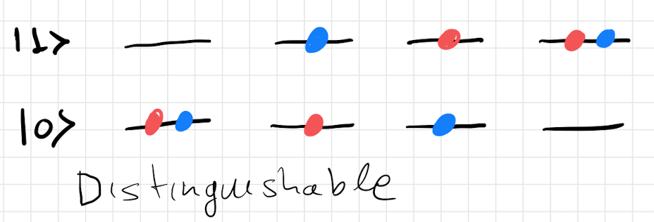
As an example of this would work. We will consider a simple system which has two single particle states $\mid 0⟩$ and $\mid 1⟩$. We then want to list the different configurations we can come up with for the three different classes of particles. The corresponding configurations are shown in figure 10.

Figure 10: The top figure shows the inequivalent configurations of two distinguishable identical particles in the two state system. The bottom does the same for identical Bosons (left) and Fermions (right).

3.4 Bosons

In this subsection we will consider a general system of non-interacting Bosons. In order to give a general description, we will denote the $r$-th single particle microstate by $\mid r⟩$ and the corresponding energy level by $E_{\mid r⟩}$. Since Bosons are indistinguishable, the microstates of a system of $N$ particles will be characterised by an infinite number of integers $\{n_{\mid r⟩}\}$ equal to the number of particles in the single particle microstate $\mid r⟩$. The integers $n_{\mid r⟩}$ are called the occupation numbers of the single particle microstates. The constraint these integers need to satisfy is,

${\displaystyle \sum _{\mid r⟩}}{n}_{\mid r⟩}=N,$ (245)

yielding the corresponding total energy,

$E_{\{n_{\mid r⟩}\}}={\displaystyle \sum _{\mid r⟩}}{n}_{\mid r⟩}{E}_{\mid r⟩}.$ (246)

The $N$-body canonical partition function can be written as,

$Z(\beta ,V,N)={\displaystyle \sum _{\{n_{\mid r⟩}\}}}{e}^{-\beta {\sum }_{\mid r⟩}{n}_{\mid r⟩}{E}_{\mid r⟩}},$ (247)

where the sum is performed over all set of integers $\{n_{\mid r⟩}\}$ satisfying the constraint (245).

This sum is highly non-trivial and the situation is significantly simplified by considering the grand canonical ensemble instead as we will need to sum over $N$. To see this simplification, we recall the relation of equation (• ‣ 1.3) between the grand canonical and the canonical partition functions,

$𝒵(\beta ,V,\mu )$ $={\displaystyle \sum _{N=0}^{\mathrm{\infty }}}{e}^{\beta \mu N}Z(\beta ,V,N)$

$={\displaystyle \sum _{N=0}^{\mathrm{\infty }}}{e}^{\beta \mu N}{\displaystyle \sum _{\begin{array}{c}\{n_{\mid r⟩}\}\\ {\sum }_{\mid r⟩}{n}_{\mid r⟩}=N\end{array}}}{e}^{-\beta {\sum }_{\mid r⟩}{n}_{\mid r⟩}{E}_{\mid r⟩}}$ (250)

$={\displaystyle \sum _{N=0}^{\mathrm{\infty }}}{\displaystyle \sum _{\begin{array}{c}\{n_{\mid r⟩}\}\\ {\sum }_{\mid r⟩}{n}_{\mid r⟩}=N\end{array}}}{e}^{-\beta {\sum }_{\mid r⟩}{n}_{\mid r⟩}(E_{\mid r⟩}-\mu )}$ (253)

$={\displaystyle \sum _{\{n_{\mid r⟩}\}}}{e}^{-\beta {\sum }_{\mid r⟩}{n}_{\mid r⟩}(E_{\mid r⟩}-\mu )}$

$={\displaystyle \prod _{\mid r⟩}}𝒵(\beta ,V,\mu ,E_{\mid r⟩}).$ (254)

In the above, we defined the grand canonical partition function corresponding to the single particle microstate $\mid r⟩$ according to,

$𝒵(\beta ,V,\mu ,E_{\mid r⟩})$ $={\displaystyle \sum _{n_{\mid r⟩}=0}^{\mathrm{\infty }}}{e}^{-\beta (E_{\mid r⟩}-\mu )n_{\mid r⟩}}$

$={\displaystyle \frac{1}{1-e^{-\beta (E_{\mid r⟩}-\mu )}}}={\displaystyle \frac{1}{1-z{e}^{-\beta E_{\mid r⟩}}}}.$ (255)

Note that in order for the infinite sum converge, the chemical potential $\mu$ has to be smaller than the smallest energy level.

After having obtained the grand canonical partition function, the probability for a particular microstate with occupation numbers $\{n_{\mid r⟩}\}$ is,

$p(\{n_{\mid r⟩}\})={\displaystyle \frac{1}{𝒵}}{e}^{-\beta {\sum }_{\mid r⟩}{n}_{\mid r⟩}(E_{\mid r⟩}-\mu )}.$ (256)

A quantity of interest is the probability to have occupation number $n_{\mid r⟩}$ in a particular microstate $\mid r⟩$. This can be obtained after summing over all occupation numbers $n_{\mid s⟩}$ with $\mid s⟩\ne \mid r⟩$. It is now easy to compute,

$p(n_{\mid r⟩})=$ ${\displaystyle \sum _{\{n_{\mid s⟩},\mid s⟩\ne \mid r⟩\}\}}}p(\{n_{\mid s⟩}\})={\displaystyle \frac{e^{-\beta (E_{\mid r⟩}-\mu )n_{\mid r⟩}}}{𝒵}}{\displaystyle \sum _{\{n_{\mid s⟩},\mid s⟩\ne \mid r⟩\}\}}}{e}^{-\beta {\sum }_{\mid s⟩\ne \mid r⟩}{n}_{\mid s⟩}(E_{\mid s⟩}-\mu )}$

$=$ ${\displaystyle \frac{e^{-\beta (E_{\mid r⟩}-\mu )n_{\mid r⟩}}}{\left({\prod }_{\mid w⟩}𝒵(\beta ,V,\mu ,E_{\mid w⟩})\right)}}{\displaystyle \prod _{\mid s⟩\ne \mid r⟩}}\left({\displaystyle \sum _{n_{\mid s⟩}=0}^{\mathrm{\infty }}}{e}^{-\beta (E_{\mid s⟩}-\mu )n_{\mid s⟩}}\right)$

$=$ ${\displaystyle \frac{e^{-\beta (E_{\mid r⟩}-\mu )n_{\mid r⟩}}}{\left({\prod }_{\mid w⟩}𝒵(\beta ,V,\mu ,E_{\mid w⟩})\right)}}{\displaystyle \prod _{\mid s⟩\ne \mid r⟩}}𝒵(\beta ,V,\mu ,E_{\mid s⟩})$

$=$ ${\displaystyle \frac{e^{-\beta (E_{\mid r⟩}-\mu )n_{\mid r⟩}}}{𝒵(\beta ,V,\mu ,E_{\mid r⟩})}}.$ (257)

The average occupation number for the state $\mid r⟩$ is then,

$⟨n_{\mid r⟩}⟩$ $={\displaystyle \sum _{n_{\mid r⟩}}}{n}_{\mid r⟩}p(n_{\mid r⟩})$

$={\displaystyle \frac{1}{\beta }}{\displaystyle \frac{\partial }{\partial \mu }}\ln 𝒵(\beta ,V,\mu ,E_{\mid r⟩})$

$={\displaystyle \frac{1}{e^{\beta (E_{\mid r⟩}-\mu )}-1}}={\displaystyle \frac{1}{z^{-1}{e}^{\beta E_{\mid r⟩}}-1}},$ (258)

which is known as the Bose-Einstein distribution.

For the grand canonical potential we can use equation (99) to write

$\mathrm{\Phi }(\beta ,V,\mu )=-k_{B}T\ln 𝒵(\beta ,V,\mu )=-k_{B}T{\displaystyle \sum _{\mid r⟩}}\ln 𝒵(\beta ,V,\mu ,E_{\mid r⟩}).$ (259)

Note that since we are summing over all single particle microstates, we can use the density of states $g(E)$ to write,

$\mathrm{\Phi }(\beta ,V,\mu )$ $=-k_{B}T{\displaystyle \int 𝑑Eg(E)\ln 𝒵(\beta ,V,\mu ,E)}$

$=k_{B}T{\displaystyle \int 𝑑Eg(E)\ln (1-z{e}^{-\beta E})}.$ (260)

We now see that all the information that is missing is the single particle density of states.

We are also going to be interested in the average energy $⟨E⟩$ of the system and the average particle number $⟨N⟩$. For these we can use the Bose-Einstein distribution (3.4) to write,

$⟨N⟩$ $={\displaystyle \sum _{\mid r⟩}}⟨n_{\mid r⟩}⟩$

$={\displaystyle \sum _{\mid r⟩}}{\displaystyle \frac{1}{e^{\beta (E_{\mid r⟩}-\mu )}-1}}$

$={\displaystyle \int 𝑑Eg(E)\frac{1}{e^{\beta (E-\mu )}-1}}$

$={\displaystyle \int 𝑑Eg(E)\frac{1}{z^{-1}{e}^{\beta E}-1}},$ (261)

and for the energy

$⟨E⟩$ $={\displaystyle \sum _{\mid r⟩}}{E}_{\mid r⟩}⟨n_{\mid r⟩}⟩$

$={\displaystyle \sum _{\mid r⟩}}{\displaystyle \frac{E_{\mid r⟩}}{e^{\beta (E_{\mid r⟩}-\mu )}-1}}$

$={\displaystyle \int 𝑑Eg(E)\frac{E}{e^{\beta (E-\mu )}-1}}$

$={\displaystyle \int 𝑑Eg(E)\frac{E}{z^{-1}{e}^{\beta E}-1}}.$ (262)

At this point, for consistency with sections 1.2.3 and 1.2.4, we note that we could had gotten these expressions by using the grand canonical partition function (3.4) in equations (1.2.4) and (1.2.4).

3.4.1 Ideal Non-Relativistic Bose Gas (High $T$)

In this subsection, we will study the ideal gas of non-relativistic Bosons in a box. In the previous subsection we considered a general system of non-interacting Bosons which populate the single particle states $\mid r⟩$. The task is then to apply what we learned in the previous subsection for the density of states (243) of single particle in a three dimensional box.

The first thing we would like to extract for our ideal gas, is its equation of state and compare it to the equation of state (135) of the classical ideal gas at high temperatures. For this reason, we will need to compute the pressure by using the grand canonical potential (3.4) in equation (96) to obtain,

$p=$ $-{\displaystyle \frac{\partial \mathrm{\Phi }}{\partial V}}=-k_{B}T{\displaystyle \int 𝑑E\ln (1-z{e}^{-\beta E})\frac{\partial }{\partial V}g(E,V)}$

$=$ $-{\displaystyle \frac{k_{B}T}{V}}{\displaystyle \int 𝑑E\ln (1-z{e}^{-\beta E})g(E,V)}$

$=$ $-{\displaystyle \frac{k_{B}T}{V}}{\displaystyle \frac{2}{3}}{\displaystyle \int 𝑑E\ln (1-z{e}^{-\beta E})\frac{\partial }{\partial E}(Eg(E,V))}$

$=$ ${\displaystyle \frac{1}{V}}{\displaystyle \frac{2}{3}}{\displaystyle \int 𝑑E\frac{E}{z^{-1}{e}^{\beta E}-1}g(E,V)}$

$=$ ${\displaystyle \frac{2}{3}}{\displaystyle \frac{⟨E⟩}{V}}\Rightarrow$

$pV=$ ${\displaystyle \frac{2}{3}}⟨E⟩.$ (263)

In the fourth line we performed an integration by parts while in the fifth line we recalled the expression of equation (3.4) for the average energy.

The right hand side of equation (3.4.1) is a function of $T$, $V$ and $\mu$ (or $z$) and so is the average particle number in equation (3.4). The plan is to now invert equation (3.4) and express the fugacity $z$ (or $\mu$) as a function of $⟨N⟩$, $V$ and $T$. This will then allow us to go back to discussing physics at fixed $⟨N⟩$, $V$ and $T$. It will also allow us to express the equation of state (3.4.1) in terms of $p$, $V$, $⟨N⟩$ and $T$ just like equation (135).

In order to make the discussion more transparent we will introduce the Bose-Einstein integral,

$g_s(z)={\displaystyle \frac{1}{\mathrm{\Gamma }(s)}}{\displaystyle {\int }_0^{\mathrm{\infty }}}𝑑x{\displaystyle \frac{x^{s-1}}{z^{-1}{e}^x-1}},$ (264)

whose Taylor expansion around $z=0$ is,

$g_s(z)={\displaystyle \sum _{m=1}^{\mathrm{\infty }}}{\displaystyle \frac{z^m}{m^s}}.$ (265)

After introducing the change of variables of integration $x=\beta E$ in the integrals of equations (3.4) and (3.4) we can write,

${\displaystyle \frac{⟨N⟩}{V}}$ $={\lambda }^{-3}{g}_{3/2}(z),$ (266)

${\displaystyle \frac{⟨E⟩}{V}}$ $={\displaystyle \frac{3}{2}}{k}_{B}T{\lambda }^{-3}{g}_{5/2}(z),$ (267)

where $\lambda$ is the de Broglie wavelength of equation (130). In order to obtain these expressions we used that $\mathrm{\Gamma }(3/2)=\sqrt{\pi }/2$ and $\mathrm{\Gamma }(5/2)=3\sqrt{\pi }/4$.

As we discussed in the previous subsection, the chemical potential should be smaller that the energy of the ground state of our system and therefore . This suggests that fugacity $z=e^{\beta \mu }$ satisfies the inequalities . It is useful to know that the function $g_s(z)$ is monotonically increasing between $g_s(0)=0$ and $g_s(1)=\zeta (s)$ where $\zeta$ is the Riemann zeta function.

We can now proceed to imagine inverting equation (266) to write,

$g_{3/2}(z)={\displaystyle \frac{⟨N⟩}{V}}{\lambda }^3.$ (268)

This expression shows that, at fixed density $⟨N⟩/V$, the fugacity $z$ has to decrease as temperature increases. This is because according to equation (130) the de Broglie wavelength $\lambda$ decreases. Therefore, we learn that as $T\to \mathrm{\infty }$ we must have $z\to 0$. In this high temperature limit we can therefore use the series (265) to keep the first couple of term and write equation (268) as,

${\displaystyle \frac{⟨N⟩}{V}}={\displaystyle \frac{z}{{\lambda }^3}}\left(1+{\displaystyle \frac{z}{2\sqrt{2}}}+𝒪(z^2)\right).$ (269)

Inverting this equation at small $z$ we find that,

$z={\displaystyle \frac{{\lambda }^3⟨N⟩}{V}}\left(1-{\displaystyle \frac{1}{2\sqrt{2}}}{\displaystyle \frac{{\lambda }^3⟨N⟩}{V}}+𝒪\left({\left({\displaystyle \frac{{\lambda }^3⟨N⟩}{V}}\right)}^2\right)\right).$ (270)

Similarly, in the high temperature limit we can expand equation (267) to obtain,

${\displaystyle \frac{⟨E⟩}{V}}$ $={\displaystyle \frac{3}{2}}{\displaystyle \frac{z}{{\lambda }^3\beta }}\left(1+{\displaystyle \frac{z}{4\sqrt{2}}}+𝒪(z^2)\right).$ (271)

We can now combine equations (271) and (270) to express $⟨E⟩$ as a function of $T$, $⟨N⟩$ and $V$. We find,

$⟨E⟩={\displaystyle \frac{3}{2}}{\displaystyle \frac{⟨N⟩}{\beta }}\left(1-{\displaystyle \frac{1}{4\sqrt{2}}}{\displaystyle \frac{{\lambda }^3⟨N⟩}{V}}+𝒪\left({\left({\displaystyle \frac{{\lambda }^3⟨N⟩}{V}}\right)}^2\right)\right).$ (272)

Using now this high temperature approximation in the equation of state (3.4.1) we obtain,

$pV=⟨N⟩k_{B}T\left(1-{\displaystyle \frac{{\lambda }^3}{4\sqrt{2}}}{\displaystyle \frac{⟨N⟩}{V}}+𝒪\left({\left({\displaystyle \frac{{\lambda }^3⟨N⟩}{V}}\right)}^2\right)\right).$ (273)

We therefore find that at leading order we recover the equation of state of the ideal (135). It is remarkable that eventhough we don’t have interactions in our gas, the corrections organise themselves according to the Virial expansion (190) with second Virial coefficient,

$B_2(T)=-{\displaystyle \frac{{\lambda }^3}{4\sqrt{2}}}.$ (274)

The corrections come from purely quantum statistics which is different from the classical statistics we used in section 2.1.

3.4.2 Ideal Non-Relativistic Bose Gas (Low $T$) - Bose-Einstein Condensation

Even more interesting is the low temperature limit of the ideal Bose gas. To understand the behaviour of the fugacity $z$ we need to go back to equation (268). Having in mind a fixed density, we now lower the temperature of the system and we observe that the right hand side increases without an upper bound. However, we know that the left hand side is bounded by precisely $g_{3/2}(1)$. Therefore, this is telling us that this equation has valid solutions for $z$ down to a specific value of temperature $T_c$ at which,

$g_{3/2}(1)$ $={\displaystyle \frac{⟨N⟩}{V}}{\left({\displaystyle \frac{2\pi {\mathrm{\hslash }}^2}{m{k}_B{T}_c}}\right)}^{3/2}\Rightarrow$

$T_c$ $={\displaystyle \frac{2\pi {\mathrm{\hslash }}^2}{k_{B}m}}{\left({\displaystyle \frac{1}{\zeta (3/2)}}{\displaystyle \frac{⟨N⟩}{V}}\right)}^{2/3}.$ (275)

The question remains, what happens at temperatures ? It would appear that if we want to keep the density fixed, we would not be able to lower the temperature below $T_c$. Another way of reading this is that if we want to lower the temperature below $T_c$, the number of particles $⟨N⟩$ would have to reduce. But where do the particles that disappear go?

The resolution of the puzzle comes from remembering that we took the continuum limit of energy spectrum which as we mentioned in section 2.1 is valid only in the limit ${\lambda }^3\ll V/N$, which is the high temperature limit! Equation (268) is telling us that the bound is saturated when we start comparing the average volume per particle $V/⟨N⟩$ with ${\lambda }^3$.

In the continuum limit, the density that we use to compute the average number of particles in equation (3.4) is given by equation (243). As we can see this does not take into account the number of particles which are sitting at the ground state with $E=0$ since $g(E)\propto E^{1/2}$. However, going back to the Bose-Einstein distribution (3.4), the number of particles we expect to have in the ground state is

$n_0={\displaystyle \frac{z}{1-z}}.$ (276)

This does blow up as we approach $z\to 1$, close to the critical temperature $T_c$. We therefore see that a macroscopically large number of particles starts populating the ground state as we approach the critical temperature. This is a kind of phase transition known as Bose-Einstein condensation.

This suggests that we should go back to our equation (266) and add the number of particles $n_0$ of the ground state that we missed in the continuum approximation. The modified equation is,

$⟨N⟩$ $=V{\lambda }^{-3}{g}_{3/2}(z)+{\displaystyle \frac{z}{1-z}}.$ (277)

This improved equation takes into account the particles sitting right at $E=0$. The above modification implies that close to the critical temperature $T_c$, we can write,

${\displaystyle \frac{n_0}{⟨N⟩}}=1-{\displaystyle \frac{V}{⟨N⟩{\lambda }^3}}\zeta \left({\displaystyle \frac{3}{2}}\right)=1-{\left({\displaystyle \frac{T}{T_c}}\right)}^{\frac{3}{2}}.$ (278)

The phenomenon of Bose-Einstein condensation leads a very unusual state highly Quantum of matter at finite temperature. It is worth going back to examining the equation of state (3.4.1) in the limit of low temperatures. Combining with equation (267) after setting $z\approx 1$, we obtain

$p=k_{B}T{\lambda }^{-3}\zeta \left({\displaystyle \frac{5}{2}}\right)\propto T^{5/2},$ (279)

which, remarkably, is independent of the density $\frac{⟨N⟩}{V}$. Such states where realised in the MIT lab in 1995, 70 years after their their prediction by Bose and Einstein (1924-1925).

3.5 Fermions

In this subsection we will discuss statistical mechanics for the case of Fermions. The first thing we would like to understand is the set of of all Quantum States we can consider for a system of $N$ non-interacting Fermions, given their statistics discussed in section 3.3.

Similarly to section 3.4, we will consider a Quantum System with single particle states $\mid r⟩$. The generic microstate of the $N$ body non-interacting system, will once again be labelled by the occupation numbers $\{n_{\mid r⟩}\}$. The only difference of the case of Bosons is that due to the Fermionic statistics $n_{\mid r⟩}=0,1$ only. Once again, we the occupation numbers need to satisfy the constraint

${\displaystyle \sum _{\mid r⟩}}{n}_{\mid r⟩}=N,$ (280)

and the corresponding energy of the state will be,

$E_{\{n_{\mid r⟩}\}}={\displaystyle \sum _{\mid r⟩}}{n}_{\mid r⟩}{E}_{\mid r⟩}.$ (281)

Having in mind a similar approach to Bosons, we will consider the grand canonical partition function,

$𝒵(\beta ,V,\mu )$ $={\displaystyle \sum _{\{n_{\mid r⟩}\}}}{e}^{-\beta (E_{\{n_{\mid r⟩}\}}-\mu N)}$

$={\displaystyle \sum _{\{n_{\mid r⟩}\}}}{e}^{-\beta {\sum }_{\mid r⟩}{n}_{\mid r⟩}(E_{\mid r⟩}-\mu )}$

$={\displaystyle \prod _{\mid r⟩}}\left({\displaystyle \sum _{n_{\mid r⟩}=0}^1}{e}^{-\beta n_{\mid r⟩}(E_{\mid r⟩}-\mu )}\right)$

$={\displaystyle \prod _{\mid r⟩}}𝒵(\beta ,V,\mu ,E_{\mid r⟩}),$ (282)

which is very similar to the expression we derived for Bosons in equation (3.4). The only difference is that for Fermions the single particle state grand canonical partition function is,

$𝒵(\beta ,V,\mu ,E_{\mid r⟩})$ $={\displaystyle \sum _{n_{\mid r⟩}=0}^1}{e}^{-\beta n_{\mid r⟩}(E_{\mid r⟩}-\mu )}=1+e^{-\beta (E_{\mid r⟩}-\mu )}$

$=1+z{e}^{-\beta E_{\mid r⟩}}.$ (283)

At this point it is worth mentioning that for the case of Fermions, we don’t have a constraint on the chemical potential $\mu$. This is due to the fact that the sum in the above equation is finite. The fugacity $z=e^{\beta \mu }$ can therefore be any positive number.

The probability $p(n_{\mid r⟩})$ for the occupation number $n_{\mid r⟩}$ for a particular state $\mid r⟩$ can be obtained by following the logic of the derivation in equation (3.4). The result is,

$p(n_{\mid r⟩})={\displaystyle \frac{1}{𝒵(\beta ,V,\mu ,E_{\mid r⟩})}}{e}^{-\beta n_{\mid r⟩}(E_{\mid r⟩}-\mu )}.$ (284)

The resulting average occupation number is then,

$⟨n_{\mid r⟩}⟩={\displaystyle \frac{1}{1+z^{-1}{e}^{\beta E_{\mid r⟩}}}},$ (285)

which is known as the Fermi-Dirac distribution. The only difference from the Bose-Einstein distribution (3.4) is a sign that makes all the difference. As opposed to the Bose-Einstein distribution, equation (285) leads to an average occupation number with .

For the grand canonical potential we can write,

$\mathrm{\Phi }(\beta ,V,\mu )$ $=-k_{B}T\ln 𝒵(\beta ,V,\mu )=-k_{B}T{\displaystyle \sum _{\mid r⟩}}\ln 𝒵(\beta ,V,\mu ,E_{\mid r⟩})$

$=-k_{B}T{\displaystyle \int 𝑑Eg(E)\ln 𝒵(\beta ,V,\mu ,E_{\mid r⟩})}$

$=-k_{B}T{\displaystyle \int 𝑑Eg(E)\ln \left(1+z{e}^{-\beta E}\right)},$ (286)

where in the first line we used equation (3.5) and inn the second line we used the definition of the density of states of equation (237). The grand canonical potential will be useful in the next section where we will consider the equation of state for a gas of free Fermions in a box.

Finally, using the Fermi-Dirac distribution we can express the expectations values of total particle number $⟨N⟩$ and energy $⟨E⟩$. We can write,

$⟨N⟩$ $={\displaystyle \sum _{\mid r⟩}}⟨n_{\mid r⟩}⟩$

$={\displaystyle \sum _{\mid r⟩}}{\displaystyle \frac{1}{1+z^{-1}{e}^{\beta E_{\mid r⟩}}}}$

$={\displaystyle \int 𝑑Eg(E)\frac{1}{1+z^{-1}{e}^{\beta E}}},$ (287)

and for the energy

$⟨E⟩$ $={\displaystyle \sum _{\mid r⟩}}{E}_{\mid r⟩}⟨n_{\mid r⟩}⟩$

$={\displaystyle \sum _{\mid r⟩}}{\displaystyle \frac{E_{\mid r⟩}}{1+z^{-1}{e}^{\beta E}}}$

$={\displaystyle \int 𝑑Eg(E)\frac{E}{1+z^{-1}{e}^{\beta E}}}.$ (288)

Of course, we could had obtained these expressions by using grand canonical partition function (3.5) in equations (1.2.4) and (1.2.4).

3.5.1 Ideal Non-Relativistic Fermi Gas (High $T$)

We are now ready to study a system of non-interacting of Fermions in a box. All we need to do is use the formulae we derived in the previous section in conjunction with the density of states of (243). The first thing we would like to consider is the equation of state which we can find by computing the pressure. Since we are in the grand canonical ensemble, we can use equation (96) with equation (3.5) to find once again,

$p=-{\displaystyle \frac{\partial \mathrm{\Phi }}{\partial V}}\Rightarrow pV={\displaystyle \frac{2}{3}}⟨E⟩.$ (289)

with the average energy as given in (3.5). Once again, this is a function of $\beta$, $V$ and $\mu$ (or $z$).We would like to express the equation of states in terms of $\beta$, $V$ and $⟨N⟩$. Similarly to the case of Bosons, we want to invert equation (3.5) and express the fugacity as a function of $\beta$, $V$ and $⟨N⟩$. Having a closer look at equations (3.5) and (3.5), we see that we can write,

${\displaystyle \frac{⟨N⟩}{V}}$ $=-{\lambda }^{-3}{g}_{3/2}(-z),$ (290)

${\displaystyle \frac{⟨E⟩}{V}}$ $=-{\displaystyle \frac{3}{2}}{k}_{B}T{\lambda }^{-3}{g}_{5/2}(-z),$ (291)

with $g_s(z)$ as defined in equation (264) and the de Broglie wavelength as in (130).

Using similar arguments with the case of the bosons, we conclude that high temperature at fixed density $\frac{⟨N⟩}{V}$ implies that the fugacity $z$ is a small positive number. In that regime we can expand the right hand side of equation (290) by using (265), to find,

${\displaystyle \frac{⟨N⟩}{V}}={\displaystyle \frac{z}{{\lambda }^3}}\left(1-{\displaystyle \frac{z}{2\sqrt{2}}}+𝒪(z^2)\right),$ (292)

which we now invert equation to find,

$z={\displaystyle \frac{{\lambda }^3⟨N⟩}{V}}\left(1+{\displaystyle \frac{1}{2\sqrt{2}}}{\displaystyle \frac{{\lambda }^3⟨N⟩}{V}}+𝒪\left({\left({\displaystyle \frac{{\lambda }^3⟨N⟩}{V}}\right)}^2\right)\right).$ (293)

A small $z$ expansion of the expression for the average energy in (291) gives,

${\displaystyle \frac{⟨E⟩}{V}}$ $={\displaystyle \frac{3}{2}}{\displaystyle \frac{z}{{\lambda }^3\beta }}\left(1-{\displaystyle \frac{z}{4\sqrt{2}}}+𝒪(z^2)\right),$ (294)

which after plugging in the approximation (293) yields,

$⟨E⟩={\displaystyle \frac{3}{2}}{\displaystyle \frac{⟨N⟩}{\beta }}\left(1+{\displaystyle \frac{1}{4\sqrt{2}}}{\displaystyle \frac{{\lambda }^3⟨N⟩}{V}}+𝒪\left({\left({\displaystyle \frac{{\lambda }^3⟨N⟩}{V}}\right)}^2\right)\right).$ (295)

We now have an expression for the average energy in terms of $\beta$, $V$ and $⟨N⟩$ that we can use in the equation of state (289) to obtain,

$pV=⟨N⟩k_{B}T\left(1+{\displaystyle \frac{{\lambda }^3}{4\sqrt{2}}}{\displaystyle \frac{⟨N⟩}{V}}+𝒪\left({\left({\displaystyle \frac{{\lambda }^3⟨N⟩}{V}}\right)}^2\right)\right).$ (296)

We therefore see that in the high temperature limit, we obtain a corrected version of the equation of state of the classical ideal gas (135). This is very similar to the high temperature limit of the equation of state (273) for Bosons except that the second Virial coefficient changes sign due to the different statistics.

3.5.2 Ideal Non-Relativistic Fermi Gas (Low $T$)

To examine the Ideal Fermi gas we go back to the Fermi-Dirac distribution (285) which we write here in terms of the chemical potential,

$⟨n_{\mid r⟩}⟩={\displaystyle \frac{1}{1+e^{\beta (E_{\mid r⟩}-\mu )}}}.$ (297)

The zero temperature limit $\beta \to \mathrm{\infty }$ is rather interesting,

(298)

giving the plot we see in figure 11.

Figure 11: A plot of the Fermi-Dirac distribution at strictly zero temperature.

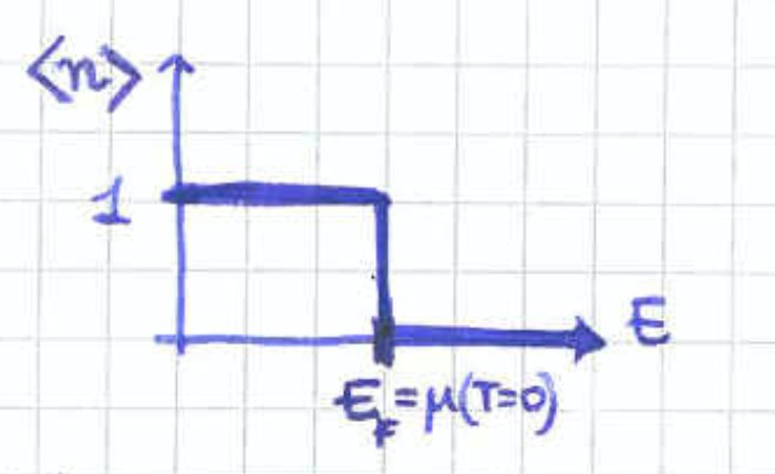
As we know, at zero temperature the only possible states is the ground state of the many body system, the state of smallest energy possible. In order to construct that state, we would populate the single particle states while respecting the statistics Fermions. This says that are only be able to put one Fermion per state forcing us to use states of successively higher energy.

From the zero temperature distribution of equation (298) we see that the highest energy states that we can use in this process is set by $\mu$. The energy of these states is called the Fermi energy of the system $E_F$. With the free particle in a box in mind, this defines a characteristic wavelength $k_F=\sqrt{2m{E}_F}/\mathrm{\hslash }$ with $p_F=\mathrm{\hslash }{k}_F$ the Fermi momentum. The single particles states which are filled have wavevectors satisfying $|\overrightarrow{k}|\le k_F$, forming the so called Fermi sea. The sphere which is the boundary of this ”Fermi ball” with $|\overrightarrow{k}|=k_F$ define the Fermi surface.

A useful task is to relate the particle number $⟨N⟩$ (or more precisely the density $⟨N⟩/V$) to $E_F$. This is achieved by using the zero temperature distribution (298) in (3.5) to obtain,

$⟨N⟩$ $={\displaystyle {\int }_0^{E_F}}𝑑Eg(E)={\displaystyle \frac{V}{6{\pi }^2}}{\left({\displaystyle \frac{2m}{{\mathrm{\hslash }}^2}}\right)}^{\frac{3}{2}}{E}_F^{\frac{3}{2}}\Rightarrow$ (299)

$E_F$ $={\displaystyle \frac{{\mathrm{\hslash }}^2}{2m}}{\left(6{\pi }^2{\displaystyle \frac{⟨N⟩}{V}}\right)}^{\frac{2}{3}}.$ (300)

We can also express the zero temperature average energy in terms of the Fermi energy,

$⟨E⟩={\displaystyle {\int }_0^{E_F}}𝑑EEg(E)={\displaystyle \frac{V}{10{\pi }^2}}{\left({\displaystyle \frac{2m}{{\mathrm{\hslash }}^2}}\right)}^{\frac{3}{2}}{E}_F^{\frac{5}{2}}.$ (301)

Using these two results in the equation of state (289) we obtain the zero temperature pressure,

$p={\displaystyle \frac{2}{5}}{\displaystyle \frac{⟨N⟩}{V}}{E}_F={\displaystyle \frac{{\mathrm{\hslash }}^2}{5m}}{(6{\pi }^2)}^{\frac{2}{3}}{\left({\displaystyle \frac{⟨N⟩}{V}}\right)}^{\frac{5}{3}}.$ (302)

The fact that the Fermionic gas retains a non-zero pressure at zero temperature is a striking feature. This behaviour is different from the classical ideal and bosonic gases where the ground state has zero energy.

Figure 12: A plot of the Fermi-Dirac distribution at small but finite temperature. The difference with the zero temperature distribution is

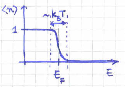
At low but finite temperatures we will employ a more intuitive approach in order to estimate the heat capacity of our Fermionic gas. We would like to compare its low temperature behaviour to what we discovered for the ideal gas which has a temperature independent heat capacity $C_V=\frac{3}{2}N{k}_B$.

As we start raising temperature from the $T=0$ distribution of figure 11, we would expect that our Fermions can absorb amounts of energy of order $k_{B}T\ll E_F$. Since all states up to $E\approx E_F$ are already occupied, we see that the only way to add this little energy to the system is to give to the Fermions which are very close to the Fermi energy. The final result would be a small deformation of the zero temperature distribution, as shown in figure 12.

The number of these particles can be found by multiplying the density of states $g(E_F,V)$ by the energy interval we expect to excite giving $\mathrm{\Delta }N=g(E_F,V)\cdot k_{B}T$. These $\mathrm{\Delta }N$ Fermions will increase the the energy of the system by,

$\mathrm{\Delta }⟨E⟩=⟨E⟩(T)-⟨E⟩(T=0)=\mathrm{\Delta }N\cdot k_{B}T=g(E_F,V)\cdot {(k_{B}T)}^2.$ (303)

This gives as an estimate for the heat capacity,

$C_V\propto k_B^{2}T.$ (304)

This tells us that the Fermionic gas has vanishing heat capacity at low temperatures. This is happening because very few electrons can absorb energy in the system due to the Fermionic statistics.