A particle moving in \(\mathbb{R}^d\) (that is, \(d\)-dimensional euclidean space) has configuration space \(\mathbb{R}^d\). We discussed the \(d=1\) example above, where we had a particle moving in the one dimensional line \(\mathbb{R}\), which we parametrized by the coordinate \(x\).

\(N\) particles moving freely in the \(\mathbb{R}^d\) have configuration space \((\mathbb{R}^{d})^N=\mathbb{R}^{dN}\). (Assuming that we can always distinguish the particles. I leave it as an amusing exercise to think what is the configuration space if you cannot distinguish the particles.)

\(N\) electrically charged particles moving in \(\mathbb{R}^d\): since particles are electrically charged they repel or attract. But this is a dynamical question, and configuration space is insensitive to such matters, it is still \(\mathbb{R}^{dN}\). One way to see this is that you can always place a set of \(N\) particles at any desired positions in \(\mathbb{R}^d\) (barring some singular points where particles overlap, so the system has infinite energy and is unphysical, but we can ignore such subtleties here). After being released, the particles will subsequently move in a manner described by the Euler-Lagrange equations, but any initial choice is permitted.

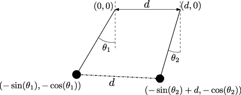
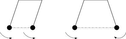
Two particles joined by a rigid rod of length \(\ell\) in \(d\)-dimensions: without the rod the configuration space is \(\mathbb{R}^{2d}\), but the rod introduces the constraint that the particles are at fixed distance \(\ell\) from each other. This can be written as \[||\vec{x}_1 - \vec{x}_2||^2 = \ell^2\] where \(\vec{x}_1\) and \(\vec{x}_2\) are the positions of the two particles in \(\mathbb{R}^d\). The configuration space is \(2d-1\) dimensional, given by the surface defined by this equation inside \(\mathbb{R}^{2d}\).

Finally, consider a rigid body in \(\mathbb{R}^3\), a desk for instance. We can view it as formed by \(~10^{27}\) atoms, joined by atomic forces. But for the purposes of classical mechanics we certainly do not care about the motion of the individual atoms (we are doing classical mechanics, not quantum mechanics, so we would get the answer wrong anyway, even if we could compute it!). Rather, for classical dynamics we can think about the classical configurations that the desk can take. And this is a six-dimensional space, given (for instance) by the position of the centre of mass of the desk, and three rotational angles.

Consider the case of a particle moving on \(\mathbb{R}^2\). The configuration space is \(\mathbb{R}^2\). There are two natural sets of coordinates in this space (although I emphasize again that any choice is valid): we could choose the ordinary Cartesian coordinates \((x,y)\), or it might be more convenient to choose polar coordinates \(r,\theta\) satisfying \[\begin{split} x & = r\cos(\theta)\, ,\\ y & = r\sin(\theta)\, . \end{split}\]

Consider instead the case of a bead attached to a circular wire of unit radius on \(\mathbb{R}^2\), defined by the equation \(x^2+y^2=1\). The configuration space is the circle, \(S^1\). A possible coordinate in this space is the angular variable \(\theta\) appearing in the description of the circle in polar coordinates.

The simplest example of the discussion so far is the free particle of mass \(m\) moving in \(d\) dimensions. Its configuration space is \(\mathbb{R}^d\), which we can parametrize using Cartesian coordinates \(x_i\). In these coordinates the kinetic energy is given by \[T = \frac{1}{2}m\sum_{i=1}^d \dot{x}_i^2\] and the potential energy \(V\) vanishes. This gives a Lagrangian \[L = T - V = \frac{1}{2}m\sum_{i=1}^d \dot{x}_i^2\] which leads to the \(d\) Euler-Lagrange equations of motion \[m\ddot{x}_i = 0 \quad \forall i\in\{1,\ldots,d\}\, .\] These equations are solved by the particle moving at constant speed, \(x_i=v_i t+b_i\), with \(v_i, b_i\) constants.

Our second example will be a pendulum moving under the influence of gravity. Our conventions will be as in figure 1: we have a mass \(m\) attached by a rigid massless rod of length \(\ell\) to a fixed point at the origin. The pendulum can swing on the \((x,y)\) plane. The configuration space of the system is \(S^1\). We choose as a coordinate the angle \(\theta\) of the rod with the downward vertical axis from the origin, measured counterclockwise. The whole system is affected by gravity, which acts downwards.

We now need to compute the kinetic and potential energy in terms of \(\theta\). The expression of the kinetic energy in the \((x,y)\) coordinates is \(\frac{1}{2}m(\dot{x}^2 + \dot{y}^2)\). In terms of \(\theta\) we have \[x = \ell \sin(\theta)\qquad \text{and}\qquad y = -\ell \cos(\theta)\, .\] This implies \(\dot{x}=\ell\cos(\theta)\dot{\theta}\) and \(\dot{y}=\ell\sin(\theta)\dot{\theta}\), so \[T = \frac{1}{2}m \ell^2 \dot{\theta}^2\,.\] The potential energy, in turn, is (up to an irrelevant additive constant) given by \[V = mgy = -mg\ell\cos(\theta)\] leading to the Lagrangian \[L = T-V = \frac{1}{2}m\ell^2\dot{\theta}^2 + mg\ell\cos(\theta)\, .\] The corresponding Euler-Lagrange equations are \[m\ell^2 \ddot{\theta} + mg\ell\sin(\theta) = 0\] or equivalently \[\ddot{\theta} + \frac{g}{\ell}\sin(\theta) = 0\, .\] The exact solution of this system requires using something known as elliptic integrals, but as a simple check of our solution, note that for small angles \(\sin(\theta)\approx \theta\), and the Euler-Lagrange equation reduces to \[\ddot{\theta} + \frac{g}{\ell}\theta = 0\] with solution \(\theta(t)=a\sin(\omega t) + b\cos(\omega t)\), where \(\omega=\sqrt{g/\ell}\), and \(a,b\) are arbitrary constants that encode initial conditions. These are the simple oscillatory solutions that one expects close to \(\theta=0\).

Consider instead a spring with a mass attached to it. The spring is attached on one end to the origin, but it is otherwise free to rotate on the \((x,y)\) plane, without friction. In this case we ignore the effect of gravity, and we assume that the spring has vanishing natural length, and constant \(\kappa\). The configuration is shown in figure 2.

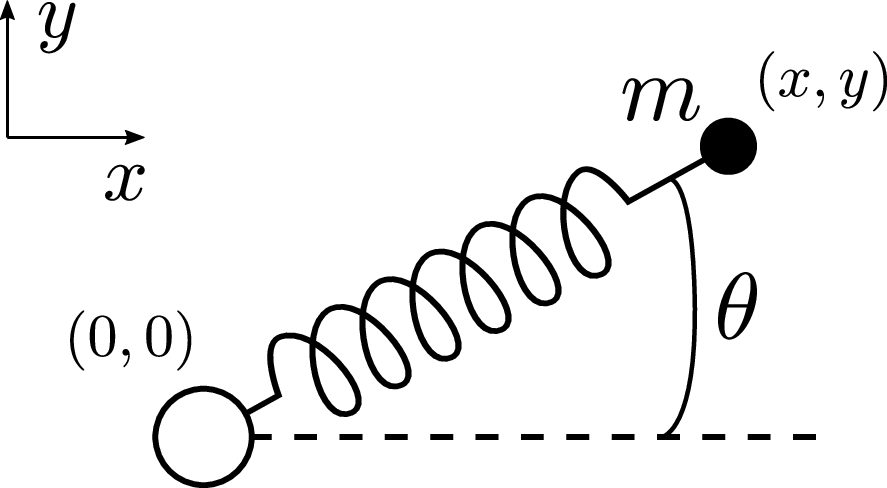
In this case the configuration space is \(\mathbb{R}^2\). It is easiest to solve the Euler-Lagrange equations in Cartesian coordinates. We have the kinetic energy \[T = \frac{1}{2}m(\dot{x}^2 + \dot{y}^2)\, .\] The potential energy is given by the square of the extension of the spring, times the spring constant. We are assuming that the natural length of the spring is 0, so we have that the extension of the spring in \(\ell = \sqrt{x^2+y^2}\). So the potential energy is \[V = \frac{1}{2}\kappa \ell^2 = \frac{1}{2}\kappa (x^2+y^2) \, .\] Putting everything together, we find that \[L = T-V = \frac{1}{2}m (\dot{x}^2+\dot{y}^2) - \frac{1}{2}\kappa (x^2+ y^2)\, .\] The Euler-Lagrange equations split into independent equations for \(x\) and \(y\), given by \[\begin{split} \ddot{x} + \frac{\kappa}{m}x &= 0\, ,\\ \ddot{y} + \frac{\kappa}{m}y & =0\, . \end{split}\] The general solution is then simply \[\begin{split} x(t)&=a_x\sin(\omega t) + b_x\cos(\omega t)\, ,\\ y(t)&=a_y\sin(\omega t) + b_y\cos(\omega t)\, , \end{split}\] with \(a_x,a_y,b_x,b_y\) constants encoding the initial conditions, and \(\omega=\sqrt{\kappa/m}\).

Let us try to solve this last example in polar coordinates \(r,\theta\). These are related to Cartesian coordinates by \[\begin{split} x & = r\cos(\theta)\, ,\\ y & = r\sin(\theta)\, . \end{split}\] Taking time derivatives, and using the Chain Rule for time derivatives, we find \[\begin{split} \dot{x} & = \dot{r}\cos(\theta) - r\sin(\theta)\dot{\theta}\, ,\\ \dot{y} & = \dot{r}\sin(\theta) + r\cos(\theta)\dot{\theta}\, . \end{split}\] A little bit of algebra then shows that \[T = \frac{1}{2}m(\dot{x}^2 + \dot{y}^2) = \frac{1}{2}m(\dot r^2 + r^2\dot{\theta}^2)\, .\] On the other hand, the potential energy is simpler. We have \[V = \frac{1}{2}\kappa (x^2+y^2) = \frac{1}{2}\kappa r^2\, .\] We thus find that the Lagrangian in polar coordinates is \[L = T-V = \frac{1}{2}m(\dot r^2 + r^2\dot{\theta}^2) - \frac{1}{2}\kappa r^2\, .\] Let us write the Euler-Lagrange equations. For the coordinate \(r\) we have \[\frac{d}{dt}\left (\frac{\partial L}{\partial {\dot r }}\right )-\frac{\partial L}{\partial r} = m\ddot{r} - mr\dot{\theta}^2 + \kappa r = 0\] while for the \(\theta\) coordinate we have \[\frac{d}{dt}\left (\frac{\partial L}{\partial {\dot \theta }}\right )-\frac{\partial L}{\partial \theta} = \frac{d}{dt}\left(mr^2\dot{\theta}\right) = 0\, .\] This equation is quite remarkable: it tells us that there is a conserved quantity in this system, given by \(mr^2\dot{\theta}\). This was not obvious at all in the Cartesian formulation of the problem,⁹ but it follows immediately in polar coordinates, since the Lagrangian does not depend on \(\theta\), only on \(\dot{\theta}\), and accordingly \(\partial L/\partial \theta=0\). We can use this knowledge to simplify the problem. Define \[J :=mr^2\dot{\theta}\, .\] This is a constant of motion, so on any given classical trajectory it is simply a real number fixed by initial conditions. We can use this knowledge to simplify the Euler-Lagrange equation for \(r\), which after replacing \(\dot{\theta}=J/mr^2\) becomes an equation purely in terms of \(r\): \[m\ddot{r} - mr\left(\frac{J}{mr^2}\right)^2 + \kappa r = m\ddot{r} - \frac{J^2}{mr^3} + \kappa r = 0\, .\]

We already found a ignorable coordinate in example [ex:rotating-spring]. We have that \(\theta\) was ignorable, and it associated generalized momentum is \[p_\theta = \frac{\partial L}{\partial\dot{\theta}} = mr^2\dot{\theta} \, .\]

An even simpler example is the free particle moving in \(d\) dimensions. In Cartesian coordinates we have \[L = T-V = \frac{1}{2} m \sum_{i=1}^d \dot{x}_i^2\, ,\] so every coordinate is ignorable. The associated generalized momenta are \[p_i = \frac{\partial L}{\partial \dot{x}_i} = m\dot{x}_i\, .\] In this case conservation of generalized momenta is simply conservation of linear momentum.

Let us look again to the free particle, but this time in two dimensions (\(d=2\)), and in polar coordinates. We have \[L = T - V = \frac{1}{2}m(\dot{r}^2 + r^2\dot{\theta}^2)\, .\] We have that \(\theta\) is ignorable. The associated conserved generalized momentum is \[p_\theta = \frac{\partial L}{\partial \dot{\theta}} = mr^2\dot{\theta}\, .\] You might recognize this as the angular momentum of the particle (that is, linear momentum \(\times\) position vector), which should indeed be conserved for the free particle.

A word on notation: when it is clear from the context which transformation we are talking about, we often write \(q_i'\) instead of \(\phi_i(\mathbf{q}, \epsilon)\). That is, we often write \[q_i \to q_i' = \ldots\] where the omitted terms are some function of \(q_i\) and \(\epsilon\).

A particle moving in \(\mathbb{R}^d\) can be described in Cartesian coordinates \(x_i\). The transformation associated to translations of the origin of coordinates in the first direction is \(x_1\to x_1 + \epsilon\), with the other coordinates constant. So we have that shifts of the coordinate system in the \(x_1\) direction are generated by \[a_i = \begin{cases} 1 & \text{for } i=1\, ,\\ 0 & \text{otherwise} \end{cases}\] and \(\dot{a}_i=0\).

Say that we have a particle moving in two dimensions, and we want to consider the finite transformations given by rotations around the origin. In Cartesian coordinates we have \[\begin{split} x & \to x\cos(\epsilon) - y\sin(\epsilon)\\ y & \to x\sin(\epsilon) + y\cos(\epsilon)\, . \end{split}\] In order to find the generators, we can derive the associated infinitesimal transformations by using the expansions \(\sin(\epsilon) = \epsilon + \mathcal{O}(\epsilon^3)\) and \(\cos(\epsilon) = 1 + \mathcal{O}(\epsilon^2)\). We find \[\begin{split} x & \to x - y\epsilon + \mathcal{O}(\epsilon^2)\\ y & \to y + x\epsilon + \mathcal{O}(\epsilon^2)\, . \end{split}\] This implies that the transformation is generated in Cartesian coordinates by \[a_x = -y \qquad ; \qquad a_y = x \qquad; \qquad \dot{a}_x = -\dot{y} \qquad ; \qquad \dot{a}_y = \dot{x}\, .\]

I emphasize that \(F(\mathbf{q},t)\) is only defined up to a constant: if some \(F(\mathbf{q},t)\) exists such that \[L' = L + \epsilon \frac{dF(\mathbf{q},t)}{dt} + \mathcal{O}(\epsilon^2)\] any other \(F'(\mathbf{q},t)=F(\mathbf{q},t)+c\) with \(c\) is a constant will also satisfy the same equation. The specific choice of \(c\) is arbitrary, and any choice will lead to correct results. In what follows I will simply pick a convenient representative \(F(\mathbf{q},t)\) — for instance \(F(\mathbf{q},t)=0\) whenever this is possible.

Whenever we have an ignorable coordinate \(q_i\), the symmetry associated to shifting it by constants, \(q_i\to q_i + c_i\), is clearly a symmetry, since by definition the coordinate does not appear in the Lagrangian, and \(\dot{q}_i\) stays invariant. So in this case \(F\) can be chosen to be 0.

As an example, consider the example of the rotating spring discussed in example [ex:rotating-spring]. In polar coordinates \((r,\theta)\), we have \[L = \frac{1}{2}m(\dot{r}^2 + r^2\dot{\theta}^2) - \frac{1}{2}\kappa r^2\, .\] In this case the \(\theta\) coordinate is ignorable, so the associated shift \(\theta\to\theta+\epsilon\) is a symmetry. The generators of the symmetry are \[a_r = 0 \qquad ; \qquad a_\theta = 1 \qquad ; \qquad \dot{a}_r = 0 \qquad ; \qquad \dot{a}_\theta = 0\, .\]

Let us study the same system as in the previous example, but now in Cartesian coordinates. We have \[L = \frac{1}{2}m (\dot{x}^2 + \dot{y}^2) - \frac{1}{2}\kappa (x^2+y^2)\, .\] The transformation \(\theta\to\theta+\epsilon\) is a rotation around the origin. Whenever \(\epsilon\ll 1\), we have \[\begin{split} x & \to x' = x - \epsilon y + \mathcal{O}(\epsilon^2)\\ y & \to y' = y + \epsilon x + \mathcal{O}(\epsilon^2)\, . \end{split}\] as we argued in example [ex:2d-in-polars]. And accordingly, for the time derivatives we have \[\begin{split} \dot{x} & \to \dot{x}' = \dot{x} - \dot{y}\epsilon + \mathcal{O}(\epsilon^2)\\ \dot{y} & \to \dot{y}' = \dot{y} + \dot{x}\epsilon + \mathcal{O}(\epsilon^2)\, . \end{split}\] Note that this transformations imply that \[x^2+y^2 \to {x}'^2+{y'}^2=(x+\epsilon y)^2+(y-\epsilon x)^2 = x^2+y^2 + \mathcal{O}(\epsilon^2)\] and similarly that \[{\dot x}^2+{\dot y}^2\to {\dot x}'^2+{\dot y}'^2={\dot x}^2+{\dot y}^2+\mathcal{O}(\epsilon^2)\] The action of the symmetry on the Lagrangian is then, to first order in \(\epsilon\): \[L \to L' = L(x', y', \dot{x}', \dot{y}') = L + \mathcal{O}(\epsilon^2)\] so we also see in this coordinate system that the rotation is a symmetry.

Note that this argument generalizes straightforwardly for any Lagrangian of the form \[L = \frac{1}{2}m(\dot{x}^2+\dot{y}^2) - V(x^2 + y^2)\] with \(V(r)\) an analytic function of \(r\), since in this case \[V(x^2+y^2+\mathcal{O}(\epsilon^2)) = V(x^2+y^2) + \mathcal{O}(\epsilon^2)\, .\]

Consider a system with Lagrangian \[L=\frac{m}{2}\left ({\dot x}^2+{\dot y}^2\right ) -y{\dot x}-\frac{1}{2}x^2\, ,\] and a transformation generated by \[\begin{aligned} x &\to & x'=x\, ,\\ y &\to & y'=y+\epsilon\, . \end{aligned}\] Then \({\dot x}'={\dot x}\) and \({\dot y}'={\dot y}\) and \[\delta L = L(x',y',{\dot x}',{\dot y}')-L(x,y,{\dot x},{\dot y})= -y'{\dot x'}+y{\dot x}=-\epsilon{\dot x}\, .\] So this is also a symmetry, this time with \(F=-x\).

Whenever the coordinate \(q_i\) is ignorable, we have a symmetry (with \(f=0\)) generated by \(q_i\to q_i+\epsilon\), leaving the other coordinates constant. That is, \[a_k = \delta_{ik} :=\begin{cases} 1 & \text{if } i = k\, .\\ 0 & \text{otherwise.} \end{cases}\] The corresponding Noether charge is then \[Q = \sum_{k=1}^N a_k\frac{\partial L}{\partial \dot{q}_i} = \sum_{k=1}^N \delta_{ki}\frac{\partial L}{\partial \dot{q}_i} = \frac{\partial L}{\partial \dot{q}_i}\] as expected.

Let us come back to the conservation of angular momentum in rotationally symmetric systems, expressed in Cartesian coordinates. Assume that we have a system with Lagrangian \[L = \frac{1}{2}m(\dot{x}^2+\dot{y}^2) - V(x^2+y^2)\, .\] We saw in example [ex:rotation-Cartesian] that rotations around the origin, which are generated by \[a_x = -y \qquad ; \qquad a_y = x\, ,\] are a symmetry of the system with \(F=0\).

Noether’s theorem then tells us that the associated charge is \[Q = a_x \frac{\partial L}{\partial \dot{x}} + a_y \frac{\partial L}{\partial \dot{y}} = m(-y\dot{x} + x\dot{y})\, .\] It is a simple exercise to show that this is indeed equal to \(mr^2\dot{\theta}\).

Finally, let us revisit example [ex:nonzero-F-symmetry]. We have a Lagrangian \[L=\frac{m}{2}\left ({\dot x}^2+{\dot y}^2\right ) -y{\dot x}-\frac{1}{2}x^2\, ,\] and a transformation generated by \[\begin{aligned} x &\to & x'=x\, ,\\ y &\to & y'=y+\epsilon\, . \end{aligned}\] That is, \(a_x=0\) and \(a_y=1\). We found in example [ex:nonzero-F-symmetry] that this transformation is a symmetry with \(F=-x\). The associated Noether charge is \[Q = a_x \frac{\partial L}{\partial \dot{x}} + a_y \frac{\partial L}{\partial \dot{y}} - F = m\dot{y} + x\, .\] We can check that this is conserved from the equations of motion, which are \[\begin{split} \frac{d}{dt}\left (\frac{\partial L}{\partial {\dot x }}\right )-\frac{\partial L}{\partial x} & = m\ddot{x} - \dot{y} + x = 0\, ,\\ \frac{d}{dt}\left (\frac{\partial L}{\partial {\dot y }}\right )-\frac{\partial L}{\partial y} & = m\ddot{y} + \dot{x} = 0\, . \end{split}\] Note in particular that the second equation is precisely \(\frac{dQ}{dt}=0\).

In this theorem \(\frac{\partial L}{\partial t}\) denotes taking the derivative of the Lagrangian with respect to time, keeping \(\mathbf{q}\) and \(\mathbf{\dot{q}}\) fixed. See note [note:time-dependent-Lagrangians] for a further discussion of this point.

Say that we have a spring that becomes weaker with time, with a spring constant \(\kappa(t)=e^{-t}\). A mass attached to the spring can then be described by a Lagrangian \[L = \frac{1}{2} m \dot{x}^2 - \frac{1}{2}\kappa(t) x^2\, .\] The resulting equation of motion is \[m\ddot{x} + \kappa(t) x = 0 \, .\] The energy of the system is \[E = \frac{1}{2} m \dot{x}^2 + \frac{1}{2}\kappa(t) x^2\, .\] Since the Lagrangian depends explicitly on time, we expect that energy is not conserved. And indeed: \[\begin{split} \frac{dE}{dt} & = m\dot{x}\ddot{x} + \kappa(t)x \dot{x} + \frac{1}{2}x^2 \frac{d\kappa(t)}{dt} \\ & = \dot{x}(m\ddot{x} + \kappa(t)x) + \frac{1}{2}x^2 \frac{d\kappa(t)}{dt} \\ & = \frac{1}{2}x^2 \frac{d\kappa(t)}{dt} \end{split}\] where in the last step we have used the equation of motion. On the other hand \[\frac{\partial L}{\partial t} = - \frac{1}{2}x^2 \frac{d\kappa(t)}{dt}\] since time appears explicitly only in \(\kappa(t)\). So we have verified that \[\frac{dE}{dt} = - \frac{\partial L}{\partial t}\, .\]

Note that our definition [def:energy] for the energy does not require the Lagrangian to have the specific form \(L=T-V\). Consider for instance the Lagrangian \[L=-m\left(\sqrt{1-\dot{x}^{2}-\dot{y}^{2}-\dot{z}^{2}}\right)\, .\] (This specific Lagrangian is in fact fairly important, as it describes the motion of a particle in \(\mathbb{R}^3\) in special relativity.) Definition [def:energy] gives \[E =\dot{x}\frac{\partial L}{\partial\dot{x}}+\dot{y}\frac{\partial L}{\partial\dot{y}}+\dot{z}\frac{\partial L}{\partial\dot{z}}-L\, .\] We have \[\dot{x}\frac{\partial L}{\partial\dot{x}}=\frac{m\dot{x}^{2}}{\sqrt{1-\dot{x}^{2}-\dot{y}^{2}-\dot{z}^{2}}},\] and similarly for \(\dot{y}\) and \(\dot{z}\). Putting everything together we find \[\begin{split} E&=\frac{m(\dot{x}^2+\dot{y}^{2}+\dot{z}^{2})}{\sqrt{1-\dot{x}^{2}-\dot{y}^{2}-\dot{z}^{2}}}+m\sqrt{1-\dot{x}^{2}-\dot{y}^{2}-\dot{z}^{2}}\\ & =\frac{m}{\sqrt{1-\dot{x}^{2}-\dot{y}^{2}-\dot{z}^{2}}}\, . \end{split}\]

Consider two pendula, each of length one with mass one, suspended a distance \(d\) apart. Connecting the masses is a spring of constant \(\kappa\) and also of natural length \(d\).

The velocity of the left hand mass is simply \(((-\cos(\theta_1){\dot \theta})_1^2+(\sin(\theta_1){\dot \theta}_1)^2)={\dot \theta}_1^2\). We get a similar result for the right hand mass so the total kinetic energy \(T\) is \[T=\frac{1}{2}\left ({\dot \theta}_1^2+{\dot \theta}_2^2\right ).\] The potential comes from gravity, which gives a contribution \(g(-\cos(\theta_1)-\cos(\theta_2))\), and from the spring. For a spring of constant \(\kappa\), its potential energy is given by \(\kappa(l-d)^2/2\), where \(l-d\) is the extension of the spring. The length \(l\) of the spring is given by Pythagoras Theorem as \[l=\sqrt{(\sin(\theta_1)-\sin(\theta_2)+d)^2+(\cos(\theta_1)-\cos(\theta_2))^2}.\] Thus the Lagrangian for the system is given by \[\begin{aligned} L&=& \frac{1}{2}\left ({\dot \theta}_1^2+{\dot \theta}_2^2\right )+g(\cos(\theta_1)+\cos(\theta_2))\\ &-&\frac{\kappa}{2}\left (\sqrt{(\sin(\theta_1)-\sin(\theta_2)+d)^2+(\cos(\theta_1)-\cos(\theta_2))^2}-d\right )^2. \end{aligned}\] Finding the exact solution to the equations of motion resulting from this Lagrangian seems hopeless. However, it is clear that the system would be happy to sit at \(\theta_1=\theta_2=0\), as this configuration minimises both the gravitational potential energy, and the spring energy since the spring would be at its natural unextended length \(d\). Let us now try to find an approximate Lagrangian which describes the system when \(\theta_i\ll 1\).

Approximating the gravitational potential is easy. \(\cos(\theta)\approx 1-\theta^2/2+O(\theta^4)\) so we can take \[-g(\cos(\theta_1)+\cos(\theta_2))=-g\left (2-\frac{\theta_1^2}{2}-\frac{\theta_2^2}{2}\right ).\] The constant term \(-2g\) can be discarded using the usual reason that additions of constants to potentials/Lagrangians has no effect. The spring potential looks more tricky to deal with, but note that to calculate \(\kappa(l-d)^2/2\) to quadratic order in the small \(\theta_i\) we only need to calculate \(l-d\) to order \(\theta_i\), since it is linear in the \(\theta_i\): \[\begin{aligned} l-d &=&\sqrt{(\sin(\theta_1)-\sin(\theta_2)+d)^2+(\cos(\theta_1)-\cos(\theta_2))^2}-d\\ &=&\sqrt{(\sin(\theta_1)-\sin(\theta_2)+d)^2}-d +O(\theta^2)\\ &=&\theta_1-\theta_2.\end{aligned}\] Finally we can write the approximate Lagrangian as \[L_{\text{approx}}=\frac{1}{2}\left ({\dot \theta}_1^2+{\dot \theta}_2^2\right )-\frac{g}{2}\left (\theta_1^2+\theta_2^2\right )-\frac{\kappa}{2}\left (\theta_1-\theta_2\right )^2.\] The equations which follow from this are \[\begin{aligned} {\ddot \theta}_1 +(g+\kappa)\theta_1 - \kappa \theta_2 &=& 0\\ {\ddot \theta}_2 - \kappa \theta_1 + (g+\kappa) \theta_2 &=&0.\end{aligned}\] If one arranges the equations of motion in this way, so that all the terms proportional to \(\theta_1\) and those proportional to \(\theta_2\) appear in columns then it is straightforward to read the elements of matrix \(A\) from the equations as \[A=\begin{pmatrix} g+\kappa & -\kappa \\ -\kappa & g+\kappa \end{pmatrix}.\] Solving for the eigenvalues of \(A\) we find that \(\lambda = g\) or \(g+2\kappa\), with eigenvectors \((1,1)\) or \((1,-1)\) respectively. So we can write the normal modes as \[\begin{pmatrix}\theta_1\\ \theta_2\end{pmatrix} = \begin{pmatrix}1\\1 \end{pmatrix} e^{\pm i\sqrt{g} t} \quad {\rm or} \quad \begin{pmatrix}\theta_1\\ \theta_2\end{pmatrix} = \begin{pmatrix}1\\-1 \end{pmatrix} e^{\pm i\sqrt{g+2\kappa} t}\] The first of these has \(\theta_1=\theta_2\) whilst the second has \(\theta_1=-\theta_2\). These two normal modes can be pictured as follows:

For the normal mode which has \(\theta_1=\theta_2\), the spring always remains exactly length \(d\) and therefore remains unextended and exerts no force. The result of this is that the angular frequency or this normal mode is \(\sqrt{g}\) which does not involve \(\kappa\) the spring constant. On the other hand, for the second normal mode the pendula move in opposite directions, and in this case the spring stretches and contracts, enhancing the effect of gravity which results in an angular frequency \(\sqrt{g+2\kappa}\) which is greater than that of the first normal mode in which only gravity plays a role.

The general solution of the system is thus given by \[\begin{split} \begin{pmatrix} \theta_1 \\ \theta_2 \end{pmatrix} & = \begin{pmatrix}1 \\ 1\end{pmatrix} \left[ \alpha^{(1)} \cos(t\sqrt{g}) + \beta^{(1)}\sin(t\sqrt{g}) \right] \\ & \phantom{=} + \begin{pmatrix}1 \\ -1\end{pmatrix} \left[ \alpha^{(2)} \cos(t\sqrt{g+2\kappa}) + \beta^{(2)}\sin(t\sqrt{g+2\kappa}) \right] \end{split}\] with \(\alpha^{(i)}\) and \(\beta^{(i)}\) arbitrary constants. To see how the general solution we found helps in practice when studying the motion of the system, let us use this solution to study what happens if we release the two masses from rest at \(t=0\) from \(\theta_1=-\theta_2=\delta\). Setting \(\theta_1=-\theta_2=\delta\) at \(t=0\) we find \[\begin{pmatrix} \delta \\ -\delta \end{pmatrix} = \begin{pmatrix} \alpha^{(1)} + \alpha^{(2)} \\ \alpha^{(1)} - \alpha^{(2)} \end{pmatrix}\] so \(\alpha^{(1)}=0\) and \(\alpha^{(2)}=\delta\). Similarly, the condition that the masses are released from rest is encoded in \[\begin{pmatrix} \dot{\theta}_1(t=0) \\ \dot{\theta}_2(t=0) \end{pmatrix} = \begin{pmatrix} 0 \\ 0 \end{pmatrix}\] which taking derivatives in our general solution is easily shown to lead to \[\begin{pmatrix} 0 \\ 0 \end{pmatrix} = \begin{pmatrix} \beta^{(1)} + \beta^{(2)} \\ \beta^{(1)} - \beta^{(2)} \end{pmatrix}\] which implies \(\beta^{(1)}=\beta^{(2)}=0\). So we find that the motion is given by \[\begin{pmatrix} \theta_1 \\ \theta_2 \end{pmatrix} = \begin{pmatrix} \delta \\ -\delta \end{pmatrix} \cos(t\sqrt{g+2\kappa})\] which is an oscillatory motion in which the masses move oppositely, without changing the centre of mass, as one might have guessed.

It is in fact possible, and we do this in section 5.2.1 below, to derive this Lagrangian density from the physics of an idealized string in the limit in which the oscillations are small. This explains the origin of the labels “density” and “tension” above. I emphasize that the uses of this Lagrangian in Mathematical Physics go well beyond explaining vibrating strings.

We could include a total derivative, or more precisely, a divergence, on the right hand side of the variation \(\delta\mathcal{L}\), as we did in the case of the point particle, but we ignore this possibility for simplicity.

The way to interpret proposition [prop:local-charge-conservation] is that it is telling us that the charge within some region changes only due to charge leaving or entering through the boundaries of the region. The current \(J_1\) measures how much charge is leaving or entering by unit time on a given boundary component.

Let us apply all this abstract discussion to our guiding example, the one-dimensional string, and the symmetry arising from \(u\) being ignorable, namely \(u\to u+\epsilon\). In this case we have \(a=1\), so the Noether current is simply given by \[{\bf J} = {\bf \Pi} = \left(\frac{\partial\mathcal{L}}{\partial u_t}, \frac{\partial\mathcal{L}}{\partial u_x}\right) = (\rho u_t, -\tau u_x) \, .\] From here, we conclude that the Noether charge \[Q = \int \!dx \, {\bf J}_{0} = \rho \int \!dx \, u_{t}\] is conserved in time, assuming that \(J_1=-\tau u_x\) vanishes at infinity (in this case, since \(\tau\) is a non-zero constant, this is equivalent to \(u_x\) vanishing at infinity). Indeed \[\frac{dQ}{dt} = \rho \int\! dx \, u_{tt} = \tau \int\! dx \, u_{xx} = \tau \bigl[u_x \bigr]_{-\infty}^{+\infty} = 0\, ,\] where in the middle step we have used the wave equation \(\rho u_{tt}=\tau u_{xx}\) for the string.

Note that we have \(d+1\) conservation equations for the energy-momentum tensor, one for each choice of “\(i\)”.

This may look a little complicated, but it is not hard to evaluate in practice. For instance, for our string we have \[T_{tt} = u_t\frac{\partial\mathcal{L}}{\partial u_t} - \mathcal{L}= \frac{\rho}{2} (u_{t})^2 + \frac{\tau}{2} (u_{x})^2\] which is indeed the energy density for the string. The rest of the components can be computed similarly, with the result \[T = \begin{pmatrix} \frac{\rho}{2} (u_{t})^2 + \frac{\tau}{2} (u_{x})^2 & -\tau u_t u_x \\ \rho u_t u_x & - \frac{\rho}{2} (u_{t})^2 - \frac{\tau}{2} (u_{x})^2 \end{pmatrix}\] The conservation laws in the case of the string are then: \[\frac{\partial T_{tt}}{\partial t} + \frac{\partial T_{tx}}{\partial x} = 0\] and similarly \[\frac{\partial T_{xt}}{\partial t} + \frac{\partial T_{xx}}{\partial x} = 0\] In order to see what these laws mean physically, let us denote the energy in the piece of string lying between \(x=a\) and \(x=b\) by \(E_{(a,b)}(t)\). Since we had that the energy density is given by \(T_{tt}\), we have that \[E_{(a,b)}=\int_{a}^{b} T_{tt}\, dx.\] The energy in this piece of string will not be conserved. It might be at rest at one time, and then a few seconds later acquire energy as a wave passes between \(x=a\) and \(x=b\), and then later, lose all its energy as the wave passes on. How the energy in this portion of the string varies is given by \[\begin{split} \frac{d}{dt}(E_{(a,b)}(t)) & = \frac{d}{dt} \int_a^b \! T_{tt}\, dx\\ & = \int_{a}^{b} \frac{\partial T_{tt}}{\partial t} \, dx \\ & = - \int_{a}^{b} \frac{\partial T_{tx}}{\partial x}\, dx \\ & = -\left[T_{tx}\right]_{a}^{b}\\ & = (T_{tx})_{x=a}-(T_{tx})_{x=b} \end{split}\] where in going from the second to the third line we have used the conservation law. In this way, the rate of change in the energy in the interval \((a,b)\) can be expressed in terms of the difference of a function evaluated at \(x=a\) and \(x=b\). If we interpret \(T_{tx}=-\tau u_t u_x\) as the flux of energy moving from left to right, then our formula can be interpreted as the rate of change of energy of the string in the interval \((a,b)\) is equal to the flux of energy coming into the segment of string from the left at \(x=a\) minus the flux of energy leaving the string segment to the right at \(x=b\).

Note that the the rate of change of \(E\), the total energy on the whole string, is given by \[\frac{dE}{dt}=\frac{d}{dt}\left (E_{(-\infty,\infty)}\right )= \tau \left [ u_t u_x \right ]_{-\infty}^\infty.\] This rate of change vanishes, so that the total energy is conserved, provided that \(u_t u_x\to 0\) as \(|x|\to \infty\). In other words, the energy is conserved provided none of it leaks away at infinity. If we disturb the string at \(t=0\) near \(x=0\), it will take an infinite amount of time before the disturbance propagates out to infinity, so indeed energy will be conserved.

The Euler-Lagrange equations are second order linear differential equations on \(\mathbf{q}(t)\) (assuming that the Lagrangian depends on \(\mathbf{q}(t)\) and \(\mathbf{\dot{q}}(t)\) only, and not higher derivatives of \(\mathbf{q}(t)\)). We can fix the integration constants that appear in solving these equations by giving the positions \(\mathbf{q}(t_0)\) and velocities \(\mathbf{\dot{q}}(t_0)\) at any chosen time \(t_0\), for some convenient choice of generalised coordinates and velocities. Once we have fixed these constants we know the behaviour of the system for all future times, so in this case we can parametrize the state at a given time \(t\) by giving \(\mathbf{q}(t)\) and \(\mathbf{\dot{q}}(t)\).

The parametrization of the physical state in terms of \(\mathbf{q}(t)\) and \(\mathbf{\dot{q}}(t)\) is not the only possible one: any parametrisation that allows us to fully fix future evolution is valid. We will see an example of a different parametrisation momentarily.

This definition for phase space sounds rather similar to the definition of configuration space (this was definition [def:configuration-space]). But note that that phase space has twice the dimension of configuration space: while configuration space encodes the (generalised) position of the system at a time \(t\), phase space encodes the generalised positions and the velocities.

Consider a particle moving in one dimension. Phase space in this case is the two dimensional plane \(\mathbb{R}^2\): one coordinate for \(x\) and one coordinate for \(\dot{x}\). Every possible point in this plane is a possible state for the particle. For instance, the point \((x,\dot{x})=(0,10)\) parametrizes a particle at the origin, moving toward positive values of \(x\). Similarly the particle moving in \(d\) dimensions has a phase space \(\mathbb{R}^{2d}\). Note that the precise form of the Lagrangian does not enter in our definition of phase space: given a point in phase space the Lagrangian will determine future evolution, but any point in phase space is acceptable as an initial condition (by definition).

Consider a particle of mass \(m\) moving in one dimension, expressed in Cartesian coordinates. Its Lagrangian is \[L(x,\dot{x}) = \frac{1}{2}m\dot{x}^2\, ,\] so its associated momentum is \[p = \frac{\partial L}{\partial \dot{x}} = m\dot{x}\, .\] We can trivially solve this equation to find \(\dot{x} = p/m\). We find that the Lagrangian for this system is thus \[L(x,p) = \frac{p^2}{2m}\] in the Hamiltonian formalism.

Let us now take a particle moving in two dimensions, expressed in polar coordinates. Its Lagrangian is \[L(\mathbf{q},\mathbf{\dot{q}}) = \frac{1}{2}m(\dot{r}^2 + r^2\dot{\theta}^2)\] so its generalised momenta are \[p_r = m\dot{r} \qquad ; \qquad p_\theta = mr^2\dot{\theta}\, .\] We can easily invert these equations, to find \(\dot{r}=p_r/m\) and \(\dot{\theta}=p_\theta/(mr^2)\). In this way we can express any function of phase space in terms of the \(\mathbf{q}\) and \(\mathbf{p}\). For instance, for the Lagrangian itself we have \[L(\mathbf{q},\mathbf{p}) = \frac{1}{2m}\left(p_r^2 + \frac{1}{r^2}p_\theta^2\right)\, .\]

Note that in the definition of the Poisson bracket the position and momenta are independent coordinates in phase space, and are treated as independent variables when taking partial derivatives: \[\frac{\partial q_i}{\partial p_j} = \frac{\partial p_i}{\partial q_j} = 0 \qquad ; \qquad \frac{\partial q_i}{\partial q_j} = \frac{\partial p_i}{\partial p_j} = \delta_{ij}\, .\]

The simplest functions in phase space that we can construct are those that give the coordinates of a point in a given basis. From the definition of the Poisson bracket, we have the fundamental brackets \[\{q_i, q_j\} = \{p_i, p_j\} = 0 \qquad ; \qquad \{q_i, p_j\} = \delta_{ij}\, .\]

I am taking a small liberty with the language here to avoid having to introduce some additional formalism: what I have just introduced is the infinitesimal version of what is commonly known as “Hamiltonian flow” in the literature, which is typically defined for finite (that is, non-infinitesimal) transformations. The finite version of the transformation is obtained by exponentiation: \[\Phi^{(a)}_f(g) = e^{a{\{\cdot,f\}}}g :=g + a\{g,f\} + \frac{a^2}{2!}\{\{g,f\},f\} + \frac{a^3}{3!}\{\{\{g,f\},f\},f\} + \ldots\]

By studying the action of \(\Phi_f^{(\epsilon)}\) on the coordinates \(\mathbf{q}\), \(\mathbf{p}\) of phase space, we can also understand \(\Phi_f^{(\epsilon)}\) as the generator of a map from phase space to itself. We have \[\begin{split} \Phi_f^{(\epsilon)}(q_i) &= q_i + \epsilon\{q_i, f\} + O(\epsilon^2) = q_i + \epsilon \frac{\partial f}{\partial p_i} + O(\epsilon^2)\\ \Phi_f^{(\epsilon)}(p_i) &= p_i + \epsilon\{p_i,f\} + O(\epsilon^2) = p_i - \epsilon \frac{\partial f}{\partial q_i} + \mathcal{O}(\epsilon^2)\, . \end{split}\] The two definitions are compatible: \[\begin{split} \Phi_f^{(\epsilon)}(g) & = g(q_1+\epsilon\{q_1,f\},\ldots,q_n+\epsilon\{q_n,f\},p_1+\epsilon\{p_1,f\},\ldots,p_n+\epsilon\{p_n,f\})\\ & = g(q_1,\ldots,q_n,p_1,\ldots,p_n) + \epsilon\sum_{i=1}^n\left(\frac{\partial g}{\partial q_i}\{q_i,f\} + \frac{\partial g}{\partial p_i}\{p_i,f\}\right) \\ & = g(q_1,\ldots,q_n,p_1,\ldots,p_n) + \epsilon\sum_{i=1}^n\left(\frac{\partial g}{\partial q_i}\frac{\partial f}{\partial p_i} - \frac{\partial g}{\partial p_i}\frac{\partial f}{\partial q_i}\right)\\ & = g + \epsilon\{g,f\} \end{split}\] where in the second line we have done a Taylor expansion, and we have omitted higher order terms in \(\epsilon\) throughout for notational simplicity.

As a simple example, consider a particle moving in one dimension. The Hamiltonian flow \(\Phi_p\) associated to the canonical momentum \(p\) acts on phase space functions as: \[\Phi_p^{(\epsilon)}(g(q,p)) = g(q,p) + \epsilon \frac{\partial g}{\partial q} + \mathcal{O}(\epsilon^2)\, .\] Alternatively, \(\Phi_p^{(\epsilon)}\) acts on the coordinate \(q\) as \(q \to q+\epsilon\), so the effect of \(\Phi_p^{(\epsilon)}\) on phase space is a uniform shift in the \(q\) direction:

We can reproduce the effect on arbitrary functions of \(q\) from this viewpoint by doing a Taylor expansion: \[g(q+\epsilon,p) = g(q,p) + \epsilon\frac{\partial g}{\partial q} + \mathcal{O}(\epsilon^2)\, .\] (You might also find it interesting to reproduce the full form of the Taylor expansion of \(f(x+a)\) around \(x\) using the exponentiated version in remark [remark:finite-flow].)

As a second example, consider a particle of unit mass moving in two dimensions, expressed in Cartesian coordinates, which we call \(q_1\) and \(q_2\). We choose the Lagrangian to be of the form \[L = \frac{1}{2}(\dot{q}_1^2 + \dot{q}_2^2) - V(q_1,q_2)\, .\] For the function generating the flow we will choose \(J=q_1\dot{q}_2 - q_2\dot{q}_1\). (Recall from example [ex:rotations-2d-Cartesian] that this function is angular momentum, which Noether’s theorem associated with rotations around the origin.) From the Lagrangian we have \(p_1=\dot{q}_1\) and \(p_2=\dot{q}_2\), so in terms of standard \((\mathbf{q},\mathbf{p})\) coordinates of phase space we have \(J(\mathbf{q},\mathbf{p})=q_1p_2-q_2p_1\). The Hamiltonian flow \(\Phi_J^{(\epsilon)}\) then acts on phase space as \[\begin{split} \Phi_{J}^{(\epsilon)}(q_1) &=q_1+\epsilon\{q_1,J\}=q_1+\epsilon\frac{\partial J}{\partial p_1}=q_1-\epsilon q_2\, ,\\ \Phi_{J}^{(\epsilon)}(q_2) &=q_2+\epsilon\{q_2,J\}=q_2+\epsilon\frac{\partial J}{\partial p_2}=q_2+\epsilon q_1\, ,\\ \Phi_{J}^{(\epsilon)}(p_1) &=p_1+\epsilon\{p_1,J\}=p_1-\epsilon\frac{\partial J}{\partial q_1}=p_1-\epsilon p_2\, ,\\ \Phi_{J}^{(\epsilon)}(p_2) &=p_2+\epsilon\{p_2,J\}=p_2-\epsilon\frac{\partial J}{\partial q_2}=p_2+\epsilon p_1\, . \end{split}\] omitting higher orders in \(\epsilon\). So the effect of \(J\) on the coordinates can be written as an infinitesimal rotation on the \(\mathbf{q}\) and the \(\mathbf{p}\) (independently) \[\begin{aligned} \Phi_J^{(\epsilon)}\begin{pmatrix}q_1\\q_2\end{pmatrix}&=\begin{pmatrix}1 & -\epsilon\\ \epsilon & 1\end{pmatrix}\begin{pmatrix}q_1\\q_2\end{pmatrix}\, ,\\ \Phi_J^{(\epsilon)}\begin{pmatrix}p_1\\p_2\end{pmatrix}&=\begin{pmatrix}1 & -\epsilon\\ \epsilon & 1\end{pmatrix}\begin{pmatrix}p_1\\p_2\end{pmatrix}\, . \end{aligned}\] For instance, the action of \(\Phi_J^{(\epsilon)}\) on the \((q_1,q_2)\) slice of phase space (which in this case has four dimensions) is as in the following picture:

Consider the harmonic oscillator in one dimension, with Lagrangian \[L = \frac{1}{2}m\dot{x}^2 - \frac{1}{2}\kappa x^2\, .\] The generalised momentum is \(p=m\dot{x}\), so the Hamiltonian for this system is \[H = \frac{1}{2m}p^2 + \frac{1}{2}\kappa x^2\, .\]

We can apply this corollary to give a very neat proof of conservation of energy: the energy, in the Hamiltonian formalism, is equal to the Hamiltonian itself. So we have that \[\begin{equation} \label{eq:energy-conservation-Hamiltonian} \frac{dH}{dt} = \frac{\partial H}{\partial t} + \{H,H\} = \frac{\partial H}{\partial t} \end{equation}\] using the fact that the Poisson bracket is antisymmetric. So, if time does not appear explicitly in the expression for the Hamiltonian, then the Hamiltonian is conserved.

A small variation of this last equation is sometimes included as part of Hamilton’s equations. From the definition of the Hamiltonian we have that \[\begin{split} \frac{\partial H(\mathbf{q},\mathbf{p},t)}{\partial t} & = \frac{\partial}{\partial t}\left(\left(\sum_{i=1}^n \dot{q}_i(\mathbf{q},\mathbf{p},t) p_i\right) - L(\mathbf{q},\mathbf{\dot{q}}(\mathbf{q},\mathbf{p},t),t)\right)\\ & = \left(\sum_{i=1}^n p_i \frac{\partial \dot{q}_i(\mathbf{q},\mathbf{p},t)}{\partial t}\right) - \frac{\partial L(\mathbf{q}, \mathbf{\dot{q}}(\mathbf{q},\mathbf{p},t), t)}{\partial t}\, . \end{split}\] Now note that \(L\) can have an explicit dependence on \(t\) through \(\mathbf{\dot{q}}\), if \(\mathbf{\dot{q}}(\mathbf{q},\mathbf{p},t)\) depends explicitly on time. Using the Chain Rule: \[\frac{\partial L(\mathbf{q}, \mathbf{\dot{q}}(\mathbf{q},\mathbf{p},t), t)}{\partial t} = \left.\frac{\partial L(\mathbf{q}, \mathbf{\dot{q}}, t)}{\partial t}\right|_{\mathbf{q},\mathbf{\dot{q}}} + \left(\sum_{i=1}^n \left.\frac{\partial L(\mathbf{q},\mathbf{\dot{q}},t)}{\partial \dot{q}_i}\right|_\mathbf{q}\frac{\partial \dot{q}_i(\mathbf{q},\mathbf{p},t)}{\partial t}\right)\] so \[\frac{\partial H(\mathbf{q},\mathbf{p},t)}{\partial t} = -\left.\frac{\partial L(\mathbf{q}, \mathbf{\dot{q}}, t)}{\partial t}\right|_{\mathbf{q},\mathbf{\dot{q}}} + \left(\sum_{i=1}^n \left(p_i - \left.\frac{\partial L(\mathbf{q},\mathbf{\dot{q}},t)}{\partial \dot{q}_i}\right|_\mathbf{q}\right) \frac{\partial \dot{q}_i(\mathbf{q},\mathbf{p},t)}{\partial t}\right)\, .\] The second term vanishes due to the definition of the generalised momentum, so we conclude that

In particular, this makes \(\eqref{eq:energy-conservation-Hamiltonian}\) compatible with theorem [thm:energy-conservation-Lagrangian].

More generally, assume that we have a function \(Q(\mathbf{q},\mathbf{p}, t)\) on phase space. We have that \(Q\) is conserved if \[\frac{dQ}{dt} = \{Q,H\} + \frac{\partial Q}{\partial t}= 0\, .\] In particular, if \(Q\) does not depend explicitly on time, we have that \(Q\) is conserved if and only if \(\{Q,H\}=0\). By antisymmetry of the Poisson bracket we can also read this condition as \[\{H,Q\} = 0\] which can be interpreted as saying that the Hamiltonian is left invariant, to first order in \(\epsilon\), by the transformation generated by \(Q\): \[\Phi_Q(H) = H + \epsilon \{Q,H\} + O(\epsilon^2) = H + O(\epsilon^2) \, .\]

A system whose Lagrangian is given by \[L=\frac{1}{2}\left ( {\dot r}^2 + r^2{\dot \theta}^2 \right )-\frac{r^2}{2}.\] We define the momenta to be \[\begin{aligned} p_r&=\frac{\partial L}{\partial {\dot r}} = {\dot r}\\ p_\theta&=\frac{\partial L}{\partial {\dot \theta}} = r^2 {\dot \theta} \end{aligned}\] so that \[\begin{aligned} {\dot r} &= p_r\\ {\dot \theta}&= \frac{p_\theta}{r^2} \end{aligned}\] The Hamiltonian is given by \[\begin{aligned} H &= p_r{\dot r}+p_\theta{\dot \theta}-\left (\frac{1}{2}\left ( {\dot r}^2 + r^2{\dot \theta}^2 \right )-\frac{r^2}{2}\right )\\ &= p_r^2 + p_\theta\left (\frac{p_\theta}{r^2}\right ) -\frac{1}{2}\left ( {p_r}^2 + r^2\left (\frac{p_\theta}{r^2}\right )^2-\frac{r^2}{2}\right )\\ &= \frac{1}{2}\left (p_r^2 +\frac{p_\theta^2}{r^2}\right )+\frac{r^2}{2}. \end{aligned}\] Hamilton’s Equations of Motion tell us that \[\begin{aligned} {\dot r} &= \frac{\partial H}{\partial p_r}=p_r\\ {\dot \theta} &= \frac{\partial H}{\partial p_\theta}=\frac{p_\theta}{r^2}\\ {\dot p_r} &= -\frac{\partial H}{\partial r} =\frac{p_\theta^2}{r^3}-r\\ {\dot p_\theta} &= -\frac{\partial H}{\partial \theta}=0. \end{aligned}\] Note that the first two equations here simply reproduce the results of expressing the \(\mathbf{q}\) in terms of the \(\mathbf{p}\)’s. This is always the case when we derive the Hamiltonian system from a Lagrangian system like above. The last equation shows that \(p_\theta\) is conserved as a result of the Hamiltonian being independent of \(\theta\). The concept of an ignorable coordinate goes over completely from the Lagrangian picture to the Hamiltonian picture. The real ‘meat’ of the dynamics is in the remaining equation for \({\dot p_r}\). Given that \(p_\theta\) is a constant and that \(p_r={\dot r}\) it can be read as \[{\ddot r} = \frac{p_\theta^2}{r^3}-r.\]

Suppose we start instead with a Hamiltonian: \[H=\frac{p^2}{2}+xp.\] Hamilton’s equations are \[\begin{aligned} {\dot x} &= \frac{\partial H}{\partial p}=p+x\\ {\dot p} &= -\frac{\partial H}{\partial x}= - p. \end{aligned}\] Solving the second equation, we have that \(p=Ae^{-t}\). Substituting this into the first equation we find \[{\dot x} - x = Ae^{-t}\] which is a linear first order differential equation. Multiplying through by the integrating factor we find \[\frac{d}{dt}\left (xe^{-t}\right ) = Ae^{-2t}\] which can be integrated to give \(x=Ce^t -Ae^{-t}/2\).

The following is a Hamiltonian for the damped harmonic oscillator: \[H=\frac{e^{-bt}p^2}{2} + \frac{e^{bt}w^2 x^2}{2}.\] Notice that \(H\) explicitly depends on time; this implies that it is not conserved, as we would expect for the damped harmonic oscillator, whose motion dies away to nothing. Hamilton’s equation of motion are \[\begin{aligned} {\dot x} &= \frac{\partial H}{\partial p} = e^{-bt}p\\ {\dot p} &= -\frac{\partial H}{\partial x} = -w^2e^{bt}x. \end{aligned}\] Differentiating the first equation with respect to \(t\), we see that \[\begin{aligned} {\ddot x} &= -be^{-bt}p+e^{-bt}{\dot p}\\ &= -b{\dot x}-w^2 x \end{aligned}\]