They often present things in a way that is slightly different to the approach being taken here.
Comments about the lecture notes are very welcome – especially if you find any mistakes and/or typos.
Classical computing
Basic gates
We will see that the ability to put a qubit in an entangled state which is a linear combination of \(|0 \rangle\) and \(|1 \rangle\), \(|\psi \rangle = \alpha |0 \rangle+ \beta |1 \rangle\), makes quantum computation qualitatively different from computation using classical bits, which are either \(0\) or \(1\). Clever algorithms can exploit this freedom to perform computations much more efficiently on a quantum computer.
To make this comparison possible, we start with a very brief review of classical computation. This is not meant as a reasonable introduction to the subject, but just to provide enough familiarity to enable you to appreciate the differences in the quantum case.
The questions we want to answer are:
What is a computation? How do we describe the process of performing a computation?
How long does it take us to perform the computation, as a function of the size of the input we’re operating on?
A simple example is the familiar procedure for adding two numbers: we add the least significant digits, carry over to the next digit if necessary, and continue; this procedure has a resource requirement that grows linearly in the number of digits.
We will consider digital computation, so we are interested in computing an integer-valued function \(f(x)\) of an integer-valued argument \(x\). This is the kind of operation carried out by actual computers. As we will see, the functions can be thought of as logical operations (combinations of AND, OR, NOT, etc); finite-precision operations with real numbers can also be represented in this way, by considering a decimal expansion of the real number as some integer.
A computation is some procedure for evaluating a given function \(f(x)\). We will use an abstract model of a computation by a circuit diagram. This is a graphical representation of a function \(f(x)\), which builds it up out of a set of simple elementary operations. This captures some features of the mode of operation of actual computers, although the specific function a given circuit computes is fixed, while a programmable computer can compute any function, which is specified by the program we input. The circuit model should not be taken too literally as a description of the physical computer, but rather as an abstract way of understanding how the desired function is built up from simpler operations. We introduce this here mainly because we will heavily use a similar graphical representation in our discussion of quantum computing.
We want to represent an integer-valued function of an integer \(x\). We represent \(x\) in binary notation, as a string of bits \(x_{n-1} x_{n-2} \ldots x_0\). This is a positional notation, so the different bits multiply powers of 2; what this means is \[x = x_{n-1} \times 2^{n-1} + x_{n-2} \times 2^{n-2} + \ldots + x_1 \times 2 + x_0 \times 2^0.\] So for example \(x = 1101 = 1 \times 2^3 + 1 \times 2^2 + 0 \times 2 + 1 = 13\).
In the model, we draw a line, representing a wire, for each bit. We draw the input as a series of wires, with the most significant bit at the top (note the difference in convention from Nielsen & Chuang).
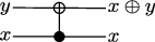
We draw a set of elementary operations as gates, acting on a sequence of bits. The gates are joined together in sequence to form the desired operation. Note circuits read left to right, with the last operation on the right, but if I write the operations as a formula they are written with the last operation to the left. For example, this circuit

constructs the function \(f(x,y) = \mathrm{NOT}(x\, \mathrm{AND}\, (\mathrm{NOT}\, y))\). (We’ll define all the gates involved in this circuit in a second.)
Let’s start by the simplest case: one bit in and one bit out. There are exactly four gates of this type, which we will describe as functions \(f\colon \{0,1\}\to \{0,1\}\):
The identity function \(f(x)=x\). Since this involves no computation we do not indicate it explicitly in the circuit model.
The NOT gate, which inverts the given value: \(f(0)=1\) and \(f(1)=0\). The name of this gate (as in some of the gates below) follows from the interpretation of the gate in terms of classical logic, thinking of 0 as “False” and 1 as “True”. An alternative useful description of this function is \(f(x)=x+1\) mod 2. We will denote NOT gates in our circuits by

The last two functions are the constant functions \(f(x)=0\) and \(f(x)=1\). We will not have much use for these functions, so we will not introduce any special notation for them.
There is one operation that is often implicitly used when designing classical circuits, which is duplicating a classical bit. We will denote this operation the FANOUT gate, and show it as a wire splitting into two:
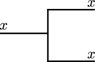
Classically this seems fairly harmless: in classical circuits we have a current flowing through a wire, so all we are doing is soldering two wires together. But, in fact, this is our first example of a gate that does not have a straightforward quantum version: by the no-cloning theorem we cannot duplicate arbitrary qubits! Below I will discuss a way of getting around this issue by using a CNOT gate (defined below) and some ancillary bits.
Let us move on to gates with two inputs, and one output. There are \(2^4=16\) possible gates of this type, but we will focus on three:
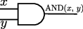
AND acts on two bits, and produces one. \(\mathrm{AND}(0,0) = \mathrm{AND}(0,1) = \mathrm{AND}(1,0) = 0\), \(\mathrm{AND}(1,1) = 1\). Note that \(\mathrm{AND}(x,y)=\mathrm{AND}(y,x)\). In this case, and in the operations below, we often write \(\mathrm{AND}(x,y)\) as \(x\mathrm{AND}y\) to avoid writing too many parenthesis. We represent this gate as
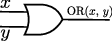
OR takes two bits as input, producing one output bit. \(\mathrm{OR}(0,0) = 0\), \(\mathrm{OR}(0,1) = \mathrm{OR}(1,0) = OR(1,1) =1\). For this gate we also have \(\mathrm{OR}(x,y)=\mathrm{OR}(y,x)\). We represent it by:
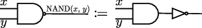
A third interesting gate is \(\mathrm{NAND}(x,y)=\mathrm{NOT}(\mathrm{AND}(x,y))\). That is, \(\mathrm{NAND}(0,0)=\mathrm{NAND}(0,1)=\mathrm{NAND}(1,0)=1\) and \(\mathrm{NAND}(1,1)=0\). We represent it by
Again we are in a situation in which something looks very sensible classically, but in fact is not doable in the quantum setting: the \(\mathrm{AND}\), \(\mathrm{OR}\) and \(\mathrm{NAND}\) gates all go from two input bits to one input bit. As functions \(f\colon \{0,1\}^2\to \{0,1\}\) they are not invertible. When talking about gates we say that they are not reversible, which we can think of as saying that the gate is throwing away some information. Quantum gates, on the other hand, will be implemented by unitary operators, which are in particular invertible.
In fact, there are good reasons to think about reversible gates in classical computers. Landauer’s principle (which I will not argue for in any detail) states that the act of erasing one bit of information from our computation in a physical computer always carries a cost: the bit cannot just disappear, but it needs to be moved into the ambient environment. Such a process consumes an amount of energy \(E\geq k_B T \log(2)\), with \(k_B\) Boltzmann’s constant, and \(T\) the temperature of the system. So, as long as we are at finite temperature, will incur some energy cost. Although modern computers are far above Landauer’s bound, it shows that theoretically there is a maximum operating efficiency for non-reversible computers. On the other hand, computers build out of purely reversible gates do not run into this bound, and theoretically do not need to dissipate energy while computing.
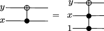
We have already seen one example of a reversible gate, the NOT gate: \(\mathrm{NOT}(\mathrm{NOT}(x))=x\), so the gate is its own inverse. Another important reversible gate is the \(\mathrm{CNOT}\) (“Controlled \(\mathrm{NOT}\)”) gate. This is a gate that takes two bits as input, know as the control bit — let us call it \(x\) — and a target bit, which we call \(y\). The \(\mathrm{CNOT}\) gate leaves \(x\) unchanged, and maps \(y\) into \(y+x\) mod 2: \(\mathrm{CNOT}(x,y)=(x,x\oplus y)\), where we have introduced the notation \[x\oplus y\mathrel{\mathop:}\mathrel{\mkern-1.2mu}=x+y\mod 2\] Equivalently, the \(\mathrm{CNOT}\) gate applies \(\mathrm{NOT}\) to \(y\) iff \(x=1\). We represent the \(\mathrm{CNOT}\) gate by:
One of the reasons why this gate is particularly important because it allows us to copy the control bit \(x\) in a reversible way by setting \(y=0\):

In doing this we need an ancillary bit. This is an extra bit initialised to a constant value, independent of the input value of the function. By convention we’ll often take the input bit to be initialised to 0.
Jumping ahead a little bit, we will see in the next section that the \(\mathrm{CNOT}\) gate can be promoted to a quantum gate. This may be a little surprising: we have just seen that the \(\mathrm{CNOT}\) gate effectively duplicates the input bit \(x\), but the no-cloning theorem tells us that quantum states cannot be cloned. How can this be? The resolution of this puzzle is that for generic input states the quantum version of the \(\mathrm{CNOT}\) gate entangles, instead of cloning: say that our input state is \(|x\rangle\otimes|0\rangle\), with \(|x\rangle=\alpha|0\rangle+\beta|1\rangle\). We can equivalently say that our input state is \(\alpha|00\rangle+\beta|10\rangle\). After applying quantum version of the the \(\mathrm{CNOT}\) gate we have \(\alpha|00\rangle+\beta|11\rangle\), which for generic \(|x\rangle\) is an entangled state, rather than the product state \(|x\rangle\otimes|x\rangle\) forbidden by the no-cloning theorem.
Given the family of input states \(|\theta\rangle\otimes|0\rangle\), with \(|\theta\rangle=\cos(\theta)|0\rangle+\sin(\theta)|1\rangle\), compute the entanglement entropy of \(\mathrm{CNOT}(|\theta\rangle\otimes|0\rangle)=\cos(\theta)|00\rangle+\sin(\theta)|11\rangle\) and \(|\theta\rangle\otimes|\theta\rangle\).
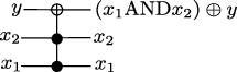
The \(\mathrm{CNOT}\) gate admits an infinite set of generalisations, the \(\mathrm{C}^n\mathrm{NOT}\) gates, which have \(n\) control bits and apply \(\mathrm{NOT}\) to a single target bit if all of the control bits are equal to 1. More algebraically: \[\mathrm{C}^n\mathrm{NOT}(x_1,\ldots,x_n,y) = (x_1,\ldots,x_n, (x_1\mathrm{AND}\ldots \mathrm{AND}x_n)\oplus y)\, .\] We can view the \(\mathrm{NOT}\) and \(\mathrm{CNOT}\) gates as the \(n=0\) and \(n=1\) special cases of this sequence. All members of this family are reversible, since \((\mathrm{C}^n\mathrm{NOT})^2=\text{id}\).
The \(n=2\) member of this family, sometimes knows as the \(\mathrm{CCNOT}\) gate, “Controlled Controlled \(\mathrm{NOT}\)”, or Toffoli gate, is particularly interesting for reasons that will become clear below. Graphically we represent this gate by
Here is the circuit diagram for the function \(f(x) = x+2\mod 16\).
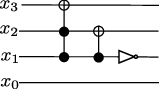
In this circuit, the right-most gate flips the second bit, adding 2 if it was initially 0. If it was initially, 1, we need to carry over to the next bit; this is implemented by the previous gate, a \(\mathrm{CNOT}\) gate, which flips the third bit if the second bit was 1. Further carries are implemented by the \(\mathrm{CCNOT}\) gate, which flip the target bit if all the control bits are 1. Because we are using just four bits, our addition works modulo 16: when we apply this circuit to \(14 = (1110)_2\) we get \(0=(0000)_2\), and similarly \(15=(1111)_2\) gets mapped to \(1=(0001)_2\).
Universal gate sets
If we wanted to promote the circuit in example [ex:add 2] to work on five bits, in order to represent the function \(f(x)=x+2\) mod 32, this could be done by using a \(\mathrm{CCCNOT}\) gate. But this is somewhat unsatisfactory: does it mean that in order to implement arbitrary logic functions in the circuit model we need to keep having to come up with arbitrarily complicated gates? Fortunately, this is not the case: we will now show that it is possible to represent any function \(f\colon \{0,1\}^n\to \{0,1\}^m\) from \(m\) bits to \(n\) bits in terms of a finite number of gates.
A finite set of gates which suffices to construct arbitrary functions \(f\colon \{0,1\}^n\to \{0,1\}^m\) is known as a Universal Gate Set (or UGS).
We will give multiple examples of universal gate sets below. In order to simplify the proof below, we write \(f\) in components \[f(x_{n-1},\ldots,x_0) = (f_{m-1}(x_{n-1},\ldots,x_0), \ldots, f_0(x_{n-1}, \ldots, x_0))\, ,\] and show that each of the components \(f_a\colon \{0,1\}^n\to\{0,1\}\), \(a=0,\ldots,m-1\), mapping \(n\) bits to a single bit can be built out of the given universal gate set. Once we show that any function \(f_a\colon \{0,1\}^n\to\{0,1\}\) can be built out of the gates in the UGS we can then build \(f\) itself as follows:
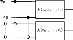
where we have shown the \(m=2\) case for simplicity. Note that in order to be able to decompose an arbitrary \(m\)-output function into single output functions we need a way of copying input bits. Here we have chosen to do so by using a \(\mathrm{CNOT}\) gate and ancillary bits, so it should be the case that \(\mathrm{CNOT}\) can also be derived from (or a member of) our universal gate set. This will be the case for all the cases we discuss below.
{\(\mathrm{NOT}\), \(\mathrm{AND}\), \(\mathrm{OR}\), \(\mathrm{CNOT}\)} are a universal gate set.
Because \(\mathrm{CNOT}\) is a member of our UGS, we can apply the splitting construction we have just discussed, and restrict our attention to functions \(f\colon \{0,1\}^n\to \{0,1\}\) producing a single bit.
We work by induction, starting from the base case \(n=1\). As we described above, there are four functions from one bit to one bit. The identity function \(f(x)=x\) and the negation \(f(x)=x\oplus 1=\mathrm{NOT}(x)\) are clearly realisable using gates in our universal gate set, so we are left with the constant functions \(f(x)=0\) and \(f(x)=1\). These can be constructed using the \(\mathrm{AND}\) gate and an ancillary bit. For instance, for \(f(x)=0\) we can take the circuit
=0.png)
and for \(f(x)=1\) the same circuit composed with a \(\mathrm{NOT}\) gate. So the set of gates given above is universal for \(n=1\).
Assume now that we know that the set of gates above is universal for \(n\) input bits, and let us show that it is then universal for \(n+1\) input bits. We can view any function \(f(x_n,x_{n-1},\ldots,x_0)\) of \(n+1\) bits as a pair of functions \(f(0,x_{n-1},\ldots,x_0)\) and \(f(1,x_{n-1},\ldots,x_0)\) of \(n\) input bits. By the inductive assumption, these are constructible in terms of the universal gate set. We can then assemble a circuit computing \(f(x_n,\ldots,x_0)\) in terms of the gates in the universal gate set and \(f(0,x_{n-1},\ldots,x_0)\), \(f(1,x_{n-1},\ldots,x_0)\) (which can in turn be assembled out of the gates in the universal gate set):
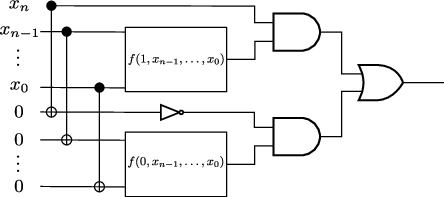
This circuit first makes a copy of all of the input bits using \(\mathrm{CNOT}\) gates and ancillary bits, and then selects the result of \(f(1,x_{n-1},\ldots,x_0)\) or \(f(0,x_{n-1},\dots,x_0)\) depending on whether \(x_n\) is 1 or 0. This is the purpose of the \(\mathrm{AND}\) gates: recall that \(0\,\mathrm{AND}\, x = 0\) and \(1\, \mathrm{AND}\, x = x\). Assume for instance that \(x_n=1\). Then the top \(\mathrm{AND}\) gate will produce the result \(f(1,x_{n-1},\ldots,x_0)\), and the bottom \(\mathrm{AND}\) gate will produce 0. Using that \(0\,\mathrm{OR}\,x=x\), the circuit then produces \(f(1,x_{n-1},\ldots,x_0)\). A similar argument shows that the circuit produces \(f(0,x_{n-1},\ldots,x_0)\) when \(x_n=0\).
Find a circuit for the Toffoli gate built from these elementary gates.
The universal gate set that we have just discussed is not minimal, and can be reduced to a smaller set without losing the universality property, as the following easy corollary shows.
{\(\mathrm{CNOT}\), \(\mathrm{AND}\)} are a universal gate set.
The \(\mathrm{NOT}\) gate can be constructed from \(\mathrm{CNOT}\) by taking the control bit to be an ancillary bit set to 1:
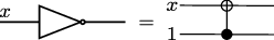
In writing this equality, and similar equalities below, we are ignoring an ancillary bit set to 1 on the left hand side, which is unaffected by the \(\mathrm{NOT}\) operation.
Once we have \(\mathrm{NOT}\) and \(\mathrm{AND}\), we can construct \(\mathrm{OR}\) using De Morgan’s law, from classical logic: \[\mathrm{NOT}\,(x\, \mathrm{OR}\, y) = (\mathrm{NOT}\, x)\, \mathrm{AND}\, (\mathrm{NOT}\, y)\, .\]
A reversible universal gate
Interestingly, it is possible to give a universal gate set consisting of a single gate, which is furthermore reversible. This is the Toffoli (or \(\mathrm{CCNOT}\)) gate. Given corollary [cy:CNOT-AND], all we need to show is that both \(\mathrm{CNOT}\) and \(\mathrm{AND}\) can be built out of the Toffoli gate. The \(\mathrm{CNOT}\) gate can be constructed similarly to the way we constructed \(\mathrm{NOT}\) in corollary [cy:CNOT-AND]:
The \(\mathrm{AND}\) gate is also not difficult to construct
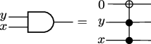
where the equality sign means in this case that after applying the \(\mathrm{CCNOT}\) gate the value of the target bit is \(x\, \mathrm{AND}\, y\).
Computational resources & Complexity
Different computational problems can have very different resource requirements. Different ways to do a computation also may require very different resources.
An algorithm is a procedure for performing a calculation; that is, some way to evaluate a function \(f(x)\). In our circuit model, different algorithms are represented by different circuits which give the same output \(f(x)\).
We want to study the resource requirements for a given circuit. There are two important resource requirements in practice: time and space. In the circuit model, time is represented by the number of elementary gates, that is the number of operations we have to perform. Space is represented by the number of bits. We will focus primarily on the first kind of resource.
A nice example is finding the greatest common divisor of two numbers \(a\) and \(b\).
A brute force approach would be to consider each number less than \(a\) and \(b\) in turn, and check whether it divides each of \(a\) and \(b\). If \(b < a\) and \(b\) has \(n\) bits, there are \(2^n\) numbers we need to check. The resource required for this computation grows exponentially in the size of the input.
Euclid’s algorithm provides a more efficient approach. We find the remainder on dividing \(a\) by \(b\), so \(a = k_1 b + r_1\). A theorem in number theory tells us gcd\((a,b) = \mathrm{gcd}(r_1, b)\). Then find the remainder on dividing \(b\) by \(r_1\), so \(b = k_2 r_1 + r_2\); by the same theorem \(\mathrm{gcd}(r_1,b) = \mathrm{gcd}(r_1, r_2)\), and carry on, computing \(r_3\) by \(r_1 = k_3 r_2 + r_3\) etc until the remainder is zero: \(r_m = k_{m+1} r_{m+1}\). Then \(\mathrm{gcd}(a,b) = \mathrm{gcd}(r_m, r_{m+1}) = r_{m+1}\). (See appendix A of Nielsen & Chuang for the relevant proofs.)
This algorithm is polynomial in the input size \(n\). This is because \(r_{i+2} < r_i/2\), so there are at most \(2n\) steps in the procedure, and (as we will not show) the divide and remainder operation at each step requires at most \(n^2\) operations, so the worst-case time to run is of order \(2n^3\).
Proof that \(r_{i+2} < r_i/2\): either \(r_{i+1} < r_i/2\), or \(r_{i+1} > r_i/2\) and hence \(r_i = 1 \times r_{i+1} + r_{i+2}\), so \(r_{i+2} = r_i - r_{i+1} < r_i/2\).
We want to classify algorithms into complexity classes, based on their resource requirements as a function of the input size.
We classify algorithms by finding an upper bound on the time it takes the algorithms to run as a function of the size \(n\) of the input to the algorithm. That is, we focus on the worst case scenario; there may be instances where the algorithm will work more quickly.
Our first two classes are
P, algorithms which run in time at most polynomial in the size of the input.
EXP, algorithms which run in time at most exponential in the size of the input.
One reason this very coarse division into P and EXP is a useful classification of algorithms is that it is believed to be independent of the details of our model of computation. This is expressed by the strong Church-Turing thesis: Any model of computation can be simulated on a universal computer with at most a polynomial increase in the number of elementary operations involved, so whether an algorithm is in P is independent of our model of computation.
For an \(n\)-bit input, a lookup table of \(f(x)\) for all values of \(x\) would have \(2^n\) entries, and looking up \(f(x)\) in the table provides an algorithm in EXP. Thus, exponential time is the worst case scenario, we don’t need anything bigger.
For a given problem, this divides algorithms into good or bad (useful and not so useful). We’d like to also classify problems, into hard and easy. For a given problem, we say that the problem is in P if we know an algorithm in P to solve it. It’s hard to prove that a problem is not in P: not knowing an efficient algorithm doesn’t mean that one doesn’t exist!
Our focus will mostly be on the time it takes to run an algorithm, but a similar classification exists when we consider space. We can define
Obviously \(\mathbf{P} \subseteq \mathbf{PSPACE}\). It is believed that \(\mathbf{P} \neq \mathbf{PSPACE}\) for problems.
An important example of a problem for which we don’t have an algorithm in P is factoring: given a number \(x\), finding its prime factors. However, if we are given a putative factorization \(x = p_1^{n_1} p_2^{n_2} \ldots\), there is a polynomial-time algorithm to multiply the RHS and see if we get \(x\).
This example motivates another class:
It is believed that \(\mathbf{P} \neq \mathbf{NP}\) for problems; this is one of the fundamental problems in the classification of computational complexity.
There are problems which are NP-complete, which means that any problem in NP can be reduced to them with only a polynomial increase in resources. Thus, finding an efficient algorithm (in P) for an NP-complete problem would allow one to solve any problem in NP efficiently, and hence would show \(\mathbf{P} = \mathbf{NP}\).
Probabilistic classical computers: For some problems, introducing a random element leads to more efficient algorithms. We allow the machine’s behaviour to also depend on the value of a random variable. This includes cases where the algorithm does not return the correct answer with certainty. This is still useful: We can either run the machine multiple times to increase the probability of correctness, or for problems in NP, use the checker algorithm to verify the solution. We define the class
Obviously \(\mathbf{P} \subseteq \mathbf{BPP}\).
Probabilistic computing is relevant to us because most quantum algorithms are also probabilistic; they don’t return the correct answer with certainty.
Anything in BPP can be efficiently solved using classical computers. The efficiency gain from quantum computing will be demonstrated by finding problems for which we do not (yet) have algorithms in BPP which can be solved efficiently on quantum computers.
Quantum Circuits
We turn now to quantum computing. We will introduce a circuit model of quantum computing, analogous to the classical one we had above. That is, we will consider operations which are built up out of a set of elementary operations.
The essence of the transition from classical to quantum computing is bits \(\to\) qubits.
The object quantum computing acts on is a state vector \(|\psi \rangle\) in a finite-dimensional Hilbert space \(\mathcal H\). We want to represent this state “in terms of qubits”. With no real loss of generality, we can take \(\mathcal H\) have dimension \(2^n\), and write is as a tensor product \(\mathcal H = \mathcal H_0 \times \ldots \times \mathcal H_{n-1}\), where each of the \(\mathcal H_i\) is a two-dimensional qubit Hilbert space with basis \(\{ |0\rangle, |1\rangle \}\). \(\mathcal H\) then has a basis \[|x\rangle = |x_{n-1} x_{n-2} \ldots x_0\rangle = |x_{n-1}\rangle \otimes |x_{n-2}\rangle \ldots \otimes |x_0\rangle\] labelled by \(n\)-bit numbers. The general state is then \[|\psi\rangle = \sum_{x=0}^{2^n-1} \psi_x |x\rangle.\] Note that specifying a quantum state requires \(2^n\) variables \(\psi_x\); compare the classical case where the state was an \(n\)-bit number \(x\).
A quantum operation is a unitary operator \(U\) on the Hilbert space \(\mathcal H\), \(U \in U(2^n)\). That \(U\) is unitary implies that the vectors \(|x'\rangle = U |x\rangle\) are orthonormal, so they form a transformed basis for \(\mathcal H\). By linearity, action of \(U\) on the computational basis states \(|x\rangle\) determines its action on any state \(|\psi\rangle\).
We will consider unitary operations on the \(n\) qubits constructed by combining a set of elementary operations which each act just on a few qubits. A key point will be to show that we can build the action of any unitary operator on \(\mathcal H\) using a simple set of elementary gate operations. That is, this is a universal model of computation, as in the classical case. This is is more non-trivial than in the classical case.
We represent the unitary operation by a circuit diagram, as in the classical case, with a wire for each qubit and the elementary operations represented as "gates" acting on one or more qubits. Unlike the classical case, the circuit is not restricted to map basis states to basis states, which gives us a much larger space of possibilities.
Quantum computation contains classical computation
Any classical computation, represented by a reversible circuit, can be implemented as a unitary operator acting on the corresponding Hilbert space \(\mathcal H\). This can be seen in two steps:
The elementary classical gates correspond to unitary operators.
A classical circuit is some combination of elementary gates acting on a few bits; this maps to a combination of the corresponding unitary operators each acting on a few qubits, defining a unitary operator on \(\mathcal H\).
The classical elementary gates were
NOT, which maps \(0 \to 1, 1 \to 0\); this corresponds to the unitary \(U = \left[ \begin{array}{cc} 0 & 1 \\ 1 & 0 \end{array} \right]\). We can see this is unitary by noting \(U^\dagger = U\), \(U^2=I\)
CNOT which maps \(00 \to 00, 01 \to 01, 10 \to 11, 11 \to 10\) (with the left bit as the control). This corresponds to the unitary (in the basis \(|00 \rangle, |01 \rangle, |10\rangle, |11\rangle\)) \[U = \left[ \begin{array}{cccc} 1 & 0 & 0 &0 \\ 0 & 1 & 0 & 0 \\ 0 & 0 & 0 & 1 \\ 0 & 0 & 1 & 0 \end{array} \right].\]
CCNOT, which acts trivially on all computational basis states except the last two, which it exchanges: \(110 \to 111, 111 \to 110\). This corresponds to an \(8 \times 8\) matrix which is the identity apart from a \(2 \times 2\) block at bottom right which is NOT, that is \(\begin{array}{cc} 0 & 1 \\ 1 & 0 \end{array}\).
This establishes that any classical computation can be performed on a quantum computer, and any reversible circuit defines a quantum unitary operation. This provides us with a rich set of examples of quantum circuits.
Example: Consider the add 2 classical circuit we had before.
Given a state \(|x \rangle\) in the computational basis the output of the circuit is \(|(x + 2) \mathrm{ mod } 2^n \rangle\). For an arbitrary quantum state \(|\psi \rangle = \sum_x \alpha_x |x \rangle\), the output is \(|\psi' \rangle = \sum_x \alpha_x |(x + 2) \mathrm{ mod } 2^n \rangle\), with the same coefficients in the superposition multiplying transformed basis states.
Basic gates
As with classical circuits, we will build the quantum circuits out of a small number of fundamental gates. To realise general unitaries, we need to slightly enlarge the gate set we considered above. Let us therefore describe some of the basic gates commonly encountered in quantum circuits and their properties.
Single-qubit gates: Classically, a single bit was either 0 or 1, and the only reversible possibilities are to do nothing, or to take the NOT of the bit. A single qubit by contrast has a two-dimensional Hilbert space, and we can act with any \(2 \times 2\) unitary matrix \(U\).
We will later use the Bloch sphere representation of a single qubit, \[|\psi \rangle = \cos (\theta/2) |0\rangle + e^{i \phi} \sin (\theta/2) |1 \rangle.\] An arbitrary unitary operator can be written up to a phase as some rotation on the Bloch sphere, \(U = e^{i \alpha} R_{\hat{n}}(\theta)\), where \(R_{\hat{n}}\) is the rotation about the axis \(\hat n\).
For now, we focus on particular examples of \(2 \times 2\) unitaries we will often use. Important examples include the Pauli matrices \[X = \left[ \begin{array}{cc} 0 & 1 \\ 1 & 0 \end{array} \right], \quad
Y = \left[ \begin{array}{cc} 0 & -i \\ i & 0 \end{array} \right] ,\quad
Z = \left[ \begin{array}{cc} 1 & 0 \\ 0 & -1 \end{array} \right].\] The first is the analogue of NOT, \(X |0\rangle = |1\rangle\), \(X |1\rangle = |0\rangle\). \(Z\) is a relative phase shift, \(Z |0\rangle = |0\rangle\), \(Z |1\rangle = - |1\rangle\), so \(\alpha |0 \rangle+ \beta |1 \rangle\) maps to \(\alpha |0 \rangle- \beta |1 \rangle\); recall that while an overall phase is irrelevant in quantum mechanics, such relative phases carry important information. Classically, something like \(Z\) would not matter, because it’s only non-trivial acting on a superposition of basis states.
[Draw pictures]
It is useful to introduce two other relative phase shifts, which are roots of \(Z\): \[S = \left[ \begin{array}{cc} 1 & 0 \\ 0 & i \end{array} \right], \quad
T = \left[ \begin{array}{cc} 1 & 0 \\ 0 & e^{i\pi/4} \end{array} \right],\] so \(T^2 = S\) and \(S^2 = Z\). Finally, a one-qubit gate we will use all the time is the Hadamard gate, \[H = \frac{1}{\sqrt{2}} \left[ \begin{array}{cc} 1 & 1 \\ 1 & -1 \end{array} \right],\] which maps \(H |0\rangle = |+\rangle = \frac{1}{\sqrt{2}} (|0 \rangle+ |1 \rangle)\), and \(H |1\rangle = |-\rangle = \frac{1}{\sqrt{2}} (|0 \rangle- |1 \rangle)\). This is really transforms the computational basis into a different basis.
Two-qubit gates: A fundamental two-qubit gate is the CNOT we saw above. The action of this gate is crucial because it creates entanglement between the two qubits. Suppose the control qubit is in a superposition of \(|0\rangle\) and \(|1\rangle\), so \[|\psi\rangle = (\alpha |0\rangle + \beta |1\rangle) \otimes |0\rangle,\] then \[CNOT |\psi\rangle = (\alpha |0\rangle \otimes |0\rangle + \beta |1\rangle \otimes |1\rangle),\] and the output is an entangled state. We can do the calculation easily in matrix notation, where \[|\psi\rangle = \left( \begin{array}{c} \alpha \\ 0 \\ \beta \\ 0 \end{array} \right), \quad CNOT |\psi\rangle = \left( \begin{array}{c} \alpha \\ 0 \\ 0\\ \beta \end{array} \right),\] but the entangled nature of the second state is much clearer in the Dirac notation. We can also have CNOT with the second bit as the control, which acts as \(X\) on the first qubit when the second qubit is \(|1\rangle\). In the matrix representation, \[U = \left[ \begin{array}{cccc} 1 & 0 & 0 &0 \\ 0 & 0 & 0 & 1 \\ 0 & 0 & 1 & 0 \\ 0 & 1 & 0 & 0 \end{array} \right],\] and we reverse the picture,
Universal quantum computation
We want to show that the circuit model, with circuits built from these basic gates, is universal for quantum computation; that is, any \(n\)-qubit unitary \(U\) can be realised as a circuit built from the basic gates. We work from the top down, starting with a general unitary and decomposing it in terms of simpler building blocks.
We first show that any unitary operation can be constructed from transformations which are non-trivial only in one \(2 \times 2\) block; that is, which act non-trivially on the two-dimensional subspace spanned by two basis states \(|s \rangle\), \(|t \rangle\).
Let’s see explicitly how it works in the \(3 \times 3\) case. In this case it should sound familiar: if my unitaries were real matrices, this would be the statement that any rotation can be written as a combination of rotations in two-dimensional planes. Given a unitary \[U = \left[ \begin{array}{ccc} a & d & g \\ b & e & h \\ c & f & j \end{array} \right],\] We will find unitaries \(U_1, U_2, U_3\) which each have a non-trivial \(2 \times 2\) block such that \(U_3 U_2 U_1 U = I\). We choose \(U_1\) to have only the first \(2 \times 2\) block non-trivial, and to be such that \[U_1U = \left[ \begin{array}{ccc} a' & d' & g' \\ b' & e' & h' \\ c' & f' & j' \end{array} \right],\] has \(b'=0\). If \(b=0\), we can simply take \(U_1 = I\). If \(b \neq 0\), we take \[U_1 = \left[ \begin{array}{ccc} \alpha^* & \beta^* & 0 \\ \beta & -\alpha & 0 \\ 0 & 0 & 1 \end{array} \right],\] with \(\alpha = \frac{a}{\sqrt{|a|^2 + |b|^2}}\), \(\beta = \frac{b}{\sqrt{|a|^2 + |b|^2}}\), so that \[b' = \beta a - \alpha b = 0.\] We then similarly choose \[U_2 = \left[ \begin{array}{ccc} \alpha^* & 0 & \beta^* \\ 0 & 1 & 0 \\ \beta & 0 & -\alpha \end{array} \right],\] such that \[U_2U_1U = \left[ \begin{array}{ccc} a'' & d'' & g'' \\ b'' & e'' & h'' \\ c'' & f'' & j'' \end{array} \right]\] has \(b'' =c'' =0\), and \(a'' =1\). This requires \(\alpha = \frac{a'}{\sqrt{|a'|^2 + |c'|^2}}\), \(\beta = \frac{c'}{\sqrt{|a'|^2 + |c'|^2}}\), so \[c'' = \beta a' - \alpha c' = 0.\] Unitarity of \(U_2 U_1 U\) then also implies \(d''=g''=0\), so \[U_2U_1U = \left[ \begin{array}{ccc} 1 & 0 & 0 \\ 0 & e'' & h'' \\ 0 & f'' & j'' \end{array} \right] \equiv U_3^\dagger,\] where \(U_3\) is non-trivial only in the bottom \(2 \times 2\) block.
If we had started with an \(N \times N\) matrix \(U\), we can find \(N-1\) unitaries \(U_1, U_2 \ldots U_{N-1}\) where \(U_i\) is non-trivial just in the first and \(i+1\)th row such that \(U_{N-1} \ldots U_1 U\) has first row and first column \(1 0 \ldots 0\), and a non-trivial \(N-1 \times N-1\) block. So by induction, we can reduce any unitary to a product of unitaries \(U_i\) which are each non-trivial just in two rows and columns. That is, the individual unitaries \(U_i\) act on a two-dimensional subspace of the Hilbert space, spanned by some pair of basis states \(|s\rangle\), \(|t\rangle\).
It takes \(\frac{1}{2} N(N-1)\) such unitaries to represent the generic \(U\). We are interested in \(U\) acting on a set of \(n\) qubits, so \(N = 2^n\), and we need \(\sim 4^n\) elementary unitaries. This indicates that the complexity of the generic unitary will be exponential in the number of qubits, just as in the classical case.
For example, in the \(4\times 4\) case, \[U = \left[ \begin{array}{cccc} * & * & 0 &0 \\ * & * & 0 &0 \\ 0 & 0 & 1 & 0 \\ 0 & 0 & 0 & 1 \end{array} \right] \left[ \begin{array}{cccc} * & 0 & * &0 \\ 0 & 1 & 0 &0 \\ * & 0 & * & 0 \\ 0 & 0 & 0 & 1 \end{array} \right] \left[ \begin{array}{cccc} * & 0 & 0 &* \\ 0 & 1 & 0 &0 \\ 0 & 0 & 1 & 0 \\ * & 0 & 0 & * \end{array} \right] \left[ \begin{array}{cccc} 1 & 0 & 0 &0 \\ 0 & * & * &0 \\ 0 & * & * & 0 \\ 0 & 0 & 0 & 1 \end{array} \right] \left[ \begin{array}{cccc} 1 & 0 & 0 &0 \\ 0 & * & 0 &* \\ 0 & 0 & 1 & 0 \\ 0 & * & 0 & * \end{array} \right] \left[ \begin{array}{cccc} 1 & 0 & 0 &0 \\ 0 & 1 & 0 &0 \\ 0 & 0 & * & * \\ 0 & 0 & * & * \end{array} \right],\] where the stars represent the entries of \(2 \times 2\) unitary matrices.
Representing the \(U_i\) as circuits
We now want to construct a circuit representations for each of the \(U_i\) acting on some subspace span\((|s\rangle, |t\rangle)\). Let’s do this first in the \(4 \times 4\) case and then generalise.
\(\left[ \begin{array}{cccc} 1 & 0 & 0 &0 \\ 0 & 1 & 0 &0 \\ 0 & 0 & * & * \\ 0 & 0 & * & * \end{array} \right]\): This acts on the subspace spanned by \(|10\rangle, |11\rangle\). We define this to be a controlled-unitary gate, by analogy to CNOT: this operates on the target bit with a \(2\times 2\) unitary \(U\) if the control bit is 1, and the identity if the control bit is 0. We represent such controlled-unitary operations as
\(\left[ \begin{array}{cccc} * & * & 0 &0 \\ * & * & 0 &0 \\ 0 & 0 & 1 & 0 \\ 0 & 0 & 0 & 1 \end{array} \right]\): This acts on the subspace spanned by \(|00\rangle, |01\rangle\). This is the same controlled-unitary, but acting if the control bit is 0 and not if the control bit is 1. This is realised by adding NOTs to the control bit:
Note that in the 2-qubit Hilbert space, NOT on \(q1\) is represented by \(\left[ \begin{array}{cccc} 0 & 0 & 1 &0 \\ 0 & 0 & 0 &1 \\ 1 & 0 & 0 & 0 \\ 0 & 1 & 0 & 0 \end{array} \right]\) (while NOT on \(q0\) is \(\left[ \begin{array}{cccc} 0 & 1 & 0 &0 \\ 1 & 0 & 0 &0 \\ 0 & 0 & 0 & 1 \\ 0 & 0 & 1 & 0 \end{array} \right]\)), so this circuit corresponds to the matrix multiplication \[\left[ \begin{array}{cccc} 0 & 0 & 1 &0 \\ 0 & 0 & 0 &1 \\ 1 & 0 & 0 & 0 \\ 0 & 1 & 0 & 0 \end{array} \right] \left[ \begin{array}{cccc} 1 & 0 & 0 &0 \\ 0 & 1 & 0 &0 \\ 0 & 0 & * & * \\ 0 & 0 & * & * \end{array} \right]\left[ \begin{array}{cccc} 0 & 0 & 1 &0 \\ 0 & 0 & 0 &1 \\ 1 & 0 & 0 & 0 \\ 0 & 1 & 0 & 0 \end{array} \right]\]
\(\left[ \begin{array}{cccc} 1 & 0 & 0 &0 \\ 0 & * & 0 &* \\ 0 & 0 & 1 & 0 \\ 0 & * & 0 & * \end{array} \right]\): This acts on the subspace spanned by \(|01\rangle, |11\rangle\). This is just the controlled-unitary with control and target reversed:
\(\left[ \begin{array}{cccc} * & 0 & * &0 \\ 0 & 1 & 0 &0 \\ * & 0 & * & 0 \\ 0 & 0 & 0 & 1 \end{array} \right]\): This acts on the subspace spanned by \(|00\rangle, |10\rangle\). Again this is a previous circuit with control and target reversed:
\(\left[ \begin{array}{cccc} 1 & 0 & 0 &0 \\ 0 & * & * &0 \\ 0 & * & * & 0 \\ 0 & 0 & 0 & 1 \end{array} \right]\): This acts on the subspace spanned by \(|01\rangle, |10\rangle\). Map this to \(|01\rangle, |11\rangle\) by CNOT, so the circuit is
\(\left[ \begin{array}{cccc} * & 0 & 0 &* \\ 0 & 1 & 0 &0 \\ 0 & 0 & 1 & 0 \\ * & 0 & 0 & * \end{array} \right]\): This acts on the subspace spanned by \(|00\rangle, |11\rangle\). Map this to \(|00\rangle, |10\rangle\) by CNOT, and use the previous circuit for that case, so the circuit is
Thus, we see that for \(4 \times 4\), we can give a circuit representation involving a new controlled-unitary operation for all the \(U_i\). To extend this to the \(N \times N\) case, first consider the matrix which acts non-trivially on the subspace spanned by \(|1\ldots 10\rangle\) and \(|1\ldots 11\rangle\): we define this to be a multiply-controlled unitary, applying some \(2 \times 2\) unitary \(U\) to the last qubit if all the others are 1, and the identity otherwise. For example, in a \(4\)-qubit Hilbert space, if we had a unitary acting in a subspace spanned by \(|1110\rangle\) and \(|1111\rangle\), this is
In general, if \(s\) and \(t\) differ in a single bit, and all the other bits are 1, this is a multiply-controlled unitary with that bit as the target. E.g., for \(|1011\rangle\) and \(|1111\rangle\), we have
If they differ in a single bit, but the others are not all 1, we need NOTs in the circuit to reverse the control bits which are 0; E.g., for \(|0001\rangle\) and \(|0101\rangle\), we have
If \(|s\rangle\) and \(|t\rangle\) don’t differ just in a single digit. We then need to transform the basis in such a way that they will. We do this by applying multiply controlled NOT gates to flip the bits of (say) \(s\) so that all but one are the same as \(t\). The process of flipping bits one by one to get from \(s\) to \(t\) is called a Gray code.
For example, if \(s = 111\) and \(t = 000\), a Gray code (not unique!) is given by the sequence \(111, 110, 100, 000\). The first step corresponds to a CCNOT gate, which flips the 3rd bit if the other bits are \(11\) (and not otherwise). In the second step, we want to flip the second qubit if the first qubit is 1 and the last is 0. This corresponds to
Then, we act on the subspace spanned by \(|100\rangle\) and \(|000\rangle\), which is acting with a controlled unitary on the first qubit when the other two are zero. In total, to act with a unitary whose \(2 \times 2\) block is spanned by \(s = 111\) and \(t = 000\), we do
In summary:
CCNOT acts like a reversible AND, so given some ancillary qubits initially set to zero, we can use CCNOT to combine the controls, so all we will need is CCNOT and controlled-unitaries.
So multiply-controlled unitaries can be realised in terms of controlled-unitary and CCNOT.
In the context of quantum computing, CCNOT is referred to as the Toffoli gate. Because of its central role in this simplification, it is sometimes taken as one of the elementary gates. However, I decided not to, so I need to reduce it to simpler components.
Verifying that this reproduces Toffoli (i.e., CCNOT) is Q7 on the homework.
In summary, at this stage
Finally, we can relate any controlled unitary to CNOT and single qubit unitaries. To do this, we need a result we will prove in the next section, that given a \(2 \times 2\) unitary \(U\), there exist unitary operators \(A, B, C\) such that \(ABC = I\) and \(U = e^{i \alpha} AXBXC\), for some phase \(\alpha\). The appropriate circuit realising the controlled-unitary is then:
Example: Controlled-\(Z\). Here we can use the fact that \(Z = HXH\) and \(HH = I\) to write a simplified version,
= .
To check this, we can do the matrix multiplication, or consider the action on the computational basis states. It is immediately obvious that \(|0 \rangle\otimes |0 \rangle\to |0 \rangle\otimes |0 \rangle\), \(|0 \rangle\otimes |1 \rangle\to |0 \rangle\otimes |1 \rangle\), as acting with \(H\) twice does nothing. If we start with \(|1 \rangle\otimes |0 \rangle\), \(H\) gives us \(|1 \rangle\otimes \frac{1}{\sqrt{2}} (|0 \rangle+ |1 \rangle)\), and the controlled-NOT gives \(|1 \rangle\otimes \frac{1}{\sqrt{2}} (|1 \rangle+ |0 \rangle)\), no effect, which \(H\) maps back to \(|1 \rangle\otimes |0 \rangle\). Starting with \(|1 \rangle\otimes |1 \rangle\), \(H\) gives us \(|1 \rangle\otimes \frac{1}{\sqrt{2}} (|0 \rangle- |1 \rangle)\), and the controlled-NOT gives \(|1 \rangle\otimes \frac{1}{\sqrt{2}} (|1 \rangle- |0 \rangle)\), so \(H\) gives \(|1 \rangle\otimes (-|1 \rangle)\), as desired.
So finally, the key result of this section is that
This universality result is quite beautiful, and remarkable: we can build arbitrary matrices acting on \(n\) qubit Hilbert spaces using just CNOT and arbitrary unitaries acting on individual qubits.
This result is not yet a complete reduction to the elementary gate set we started with. In the next section, we will consider the single qubit unitaries in more detail, and see that we can approximate a given unitary arbitrarily closely using a discrete set of transformations.
Complexity: Before turning to this, we consider the dependence of the number of gates on the number of qubits. The most important factor comes from the first step, where we broke \(U\) up into unitaries \(U_i\) with a single non-trivial \(2 \times 2\) block. We saw that this generically involves \(\frac{1}{2} N(N-1)\) unitaries \(U_i\). As \(N = 2^n\), this is exponential in the number of qubits, \(\sim 2^{2n}\). The Gray code can require \(n\) C\(^{n-1}\)NOTs, and turning these multiply controlled unitaries into controlled unitaries requires \(n\) CCNOT gates, so overall the typical \(U\) needs of order \(n^2 2^{2n}\) operations, exponential in the number of qubits. Dealing with the single-qubit unitaries will change the coefficient, but will not introduce any additional scaling with \(n\).
Our focus will be on identifying problems which do have tractable implementations in the quantum circuit model. The complexity class corresponding to this is
Quantum computing is at least as powerful as classical computing, as any polynomial-size reversible classical circuit could be implemented on qubits. so BPP \(\subseteq\) BQP. The key question in quantum computing is if there are interesting problems with solutions in BQP not in BPP.
Single-qubit unitaries
Above, we reduced arbitrary unitary operators on the Hilbert space of \(n\) qubits to a combination of CNOT operations and single-qubit unitaries. Now let us discuss the single-qubit unitaries. We want to represent these as a product of a set of elementary gates. Unlike in classical computation, where the single-bit operations were inherently discrete, we still have a continuous family of single-qubit unitaries to consider. The continuity of quantum operations is an essential difference from classical operations.
A key point is then that we can approximate a continuous operation by a product of a set of elementary operations. A useful example is provided by \(1 \times 1\) unitaries, \(U = e^{i \theta}\). The space of such unitaries is rotations in the plane, that is the unit circle \(S^1\). Given a rotation by some angle \(\alpha\) which is not a rational multiple of \(\pi\), The set \(\{ n \alpha | n \in \mathbb{Z} \}\) is dense in the circle. That is, we can approximate any rotation to any accuracy we wish by taking \(n\) rotations by \(\alpha\) for some \(n\).
We now show that the same is true for \(2 \times 2\) unitaries: they can be thought of as rotations of the sphere, and an arbitrary rotation can be approximated by products of elementary rotations.
Single-qubit unitaries are rotations in the Bloch sphere representation: In the Bloch sphere representation, \[\hat \rho = \frac{1}{2} (I + \vec r \cdot \vec \sigma) = \frac{1}{2} (I + x X + y Y + z Z),\] a pure state is specified by a vector \(\vec r\) on the unit two-sphere. A unitary transformation \(U\) acts as \(\rho \to U \rho U^\dagger\). In question 4 on the problem sheet, you show that the unitary transformation \[R_{\hat n}(\theta) = \cos(\theta/2)I - i \sin(\theta/2) (n_x X + n_y Y + n_z Z)\] corresponds to a rotation of \(\vec r\) by an angle \(\theta\) around the axis \(\vec n\) in \(\mathbb R^3\). In particular, we can think of the Pauli matrices \(X\), \(Y\), \(Z\) as generating rotations around the \(x, y, z\) axes: \[R_x(\theta) = e^{-i \theta X/2} = \cos \frac{\theta}{2} I - i \sin \frac{\theta}{2} X = \left( \begin{array}{cc} \cos \theta/2 & - i \sin \theta/2 \\ -i \sin \theta/2 & \cos \theta/2 \end{array} \right)\] \[R_y(\theta) = e^{-i \theta Y/2} = \cos \frac{\theta}{2} I - i \sin \frac{\theta}{2} Y = \left( \begin{array}{cc} \cos \theta/2 & - \sin \theta/2 \\ \sin \theta/2 & \cos \theta/2 \end{array} \right)\] \[R_z(\theta) = e^{-i \theta Z/2} = \cos \frac{\theta}{2} I - i \sin \frac{\theta}{2} Z = \left( \begin{array}{cc} e^{-i \theta/2} & 0 \\ 0 & e^{i \theta/2} \end{array} \right)\]
We want to show that any single-qubit unitary \(U\) can be written as \(U = e^{i \alpha} R_{\hat n}(\theta)\) for some choice of phase \(\alpha\), axis \(\hat n\) and angle \(\theta\). Note that the phase \(\alpha\) drops out of the action on \(\hat \rho\): \[U: \hat \rho \to U \hat \rho U^\dagger = R^\dagger_{\hat n}(\theta)\hat \rho R_{\hat n}(\theta),\] so the rotation of the Bloch sphere is the essential physical part of the unitary transformation.
To see this, let’s work out a parametrisation of arbitrary unitaries. Write \(U\) as \[U = \left( \begin{array}{cc} \sigma & \beta \\ \gamma & \delta \end{array} \right)\] The requirement that the first row is a unit vector implies \(|\sigma|^2 + |\beta|^2 =1\), so \((\sigma, \beta) = (e^{i \phi_1} \cos (\theta/2), -e^{i \phi_2} \sin (\theta/2))\) for some reals \(\theta, \phi_1, \phi_2\). Requiring that the first column is also a unit vector gives \(|\sigma|^2 + |\gamma|^2 = 1\), so \(\gamma = e^{i \phi_3} \sin \theta/2\), and making the second row a unit vector \(|\gamma|^2 + |\delta|^2 = 1\), so \(\delta = e^{i \phi_4} \cos \theta/2\). Thus, \[U = \left( \begin{array}{cc} e^{i \phi_1} \cos \theta/2 & -e^{i \phi_2} \sin \theta/2 \\ e^{i \phi_3} \sin \theta/2 & e^{i \phi_4} \cos \theta/2 \end{array} \right) .\] To make the two rows orthogonal, we need \(\phi_1 - \phi_3 = \phi_2 - \phi_4 = -\varphi_2\). To make the two columns orthogonal, we need \(\phi_1 - \phi_2 = \phi_3 - \phi_4 = - \varphi_1\). These can be solved by writing \[\begin{aligned}
\phi_1 &=& \alpha - \varphi_1 /2 - \varphi_2 /2 \\
\phi_2 &=& \alpha - \varphi_1 /2 + \varphi_2 /2 \\
\phi_3 &=& \alpha + \varphi_1 /2 - \varphi_2 /2 \\
\phi_4 &=& \alpha + \varphi_1 /2 + \varphi_2 /2 \end{aligned}\] Thus a convenient parametrisation of an arbitrary unitary \(U \in U(2)\) is \[U = e^{i \alpha} \left( \begin{array}{cc} e^{-i \varphi_1 /2 - i \varphi_2 /2} \cos \theta/2 & -e^{-i \varphi_1 /2+ i \varphi_2/2} \sin \theta/2 \\ e^{i \varphi_1 /2 - i \varphi_2/2 } \sin \theta/2 & e^{i \varphi_1 /2 + i \varphi_2/2 } \cos \theta/2 \end{array} \right) .\] This is equivalent to \[U = e^{i \alpha} \left( \begin{array}{cc} e^{-i \varphi_1 /2} & 0 \\ 0 & e^{i \varphi_1 /2} \end{array} \right) \left( \begin{array}{cc} \cos \theta/2 & -\sin \theta/2 \\ \sin \theta/2 & \cos \theta/2 \end{array} \right) \left( \begin{array}{cc} e^{-i \varphi_2 /2} & 0 \\ 0 & e^{i \varphi_2 /2} \end{array} \right)\] which is just \[U = e^{i \alpha} R_z(\varphi_1) R_y(\theta) R_z(\varphi_2)\] This product of three rotations is itself a rotation, so this establishes that any unitary \(U\) can be written as a rotation in the Bloch sphere up to an overall phase. This representation of the unitary has a useful generalisation: given two non-parallel unit vectors \(n, m\), any unitary can be written as \[U = e^{i \alpha} R_n(\beta) R_m(\gamma) R_n(\delta)\] for some values of \(\alpha, \beta, \gamma, \delta\). The proof is left as an exercise.
We can now demonstrate the result we used earlier: Given a \(2 \times 2\) unitary \(U\), there exist unitary operators \(A, B, C\) such that \(ABC = I\) and \(U = e^{i \alpha} AXBXC\), for some phase \(\alpha\). This is simply achieved by setting \[A = R_z(\varphi_1) R_y(\theta/2), \quad B = R_y(-\theta/2) R_z(-(\varphi_1 + \varphi_2)/2), \quad C = R_z((\varphi_2-\varphi_1)/2.\] Clearly \(ABC = I\). The crucial point is \[XBX = XR_y(-\theta/2)X XR_z(-(\varphi_1 + \varphi_2)/2)X = R_y( \theta/2) R_z((\varphi_1 + \varphi_2)/2),\] which you should check; then \(U = e^{i \alpha} R_z(\varphi_1) R_y(\theta) R_z(\varphi_2) = e^{i \alpha} AXBXC\).
Single-qubit unitaries in terms of elementary gates: We wanted to show that we could approximately build any single-qubit unitary by a combination of our elementary gates. Unitaries are rotations in the Bloch sphere. The Bloch sphere rotation can be written as a combination of three rotations \(R_n(\beta) R_m(\gamma) R_n(\delta)\), so if we can construct rotations \(R_n(\theta_1)\), \(R_m(\theta_2)\) about any two distinct axes, where \(\theta_1 /2\pi, \theta_2/ 2\pi\) are not rational multiples of \(\pi\), we can use these to construct approximations of \(R_n(\beta)\), \(R_m(\gamma)\) for arbitrary angles, and hence approximately recover an arbitrary unitary.
We wanted to use as elementary gates \(T\) and \(H\). Now \[T = \left( \begin{array}{cc} 1 & 0 \\ 0 & e^{i \pi/4} \end{array} \right) = e^{i \pi/8} \left( \begin{array}{cc} e^{-i\pi/8} & 0 \\ 0 & e^{i \pi/8} \end{array} \right) = e^{i \pi/8} R_z (\pi/4),\] and \[H = \frac{1}{\sqrt{2}} \left( \begin{array}{cc} 1 & 1 \\ 1 & -1 \end{array} \right) = \frac{1}{\sqrt{2}} (X+Z) = -i R_n(\pi),\] where \(n = \frac{1}{\sqrt{2}}(1,0,1)\). These are rational rotations, but \[HT = -i e^{i \pi/8} \frac{1}{\sqrt{2}} \left( \begin{array}{cc} \sin \pi/8 + i \cos \pi/8 & -\sin \pi/8 + i \cos \pi/8 \\ \sin \pi/8 + i \cos \pi/8 & \sin \pi/8 - i \cos \pi/8 \end{array} \right) = - i e^{\pi/8} R_n(\theta),\] where \[R_n(\theta) = \frac{1}{\sqrt{2}} \sin \pi/8 I + i \frac{1}{\sqrt{2}} \cos \pi/8 ( X + \tan \pi/8 Y + Z),\] so \(\cos \theta = \frac{1}{\sqrt{2}} \sin \pi/8\) and \(n = [1 + \tan^2 \pi/8]^{-1/2} (1, \tan \pi/8, 1)\). This gives an irrational angle \(\theta\). Similarly \[TH = -i e^{i \pi/8} \frac{1}{\sqrt{2}} \left( \begin{array}{cc} \sin \pi/8 + i \cos \pi/8 & \sin \pi/8 + i \cos \pi/8 \\ -\sin \pi/8 + i \cos \pi/8 & \sin \pi/8 - i \cos \pi/8 \end{array} \right) = - i e^{\pi/8} R_m(\theta),\] where \[R_m(\theta) = \frac{1}{\sqrt{2}} \sin \pi/8 I + i \frac{1}{\sqrt{2}} \cos \pi/8 ( X - \tan \pi/8 Y + Z),\] so \(\cos \theta = \frac{1}{\sqrt{2}} \sin \pi/8\) and \(n = [1 + \tan^2 \pi/8]^{-1/2} (1, -\tan \pi/8, 1)\). This is again a rotation about an irrational angle, in a different axis. Thus, \((HT)^k (TH)^l (HT)^m\) for appropriate integers \(k, l, m\) can approximate any rotation in the Bloch sphere, and hence any single-qubit unitary, up to an irrelevant overall phase.
Thus, all we need is \(H\), \(T\) and CNOT; we can build any desired unitary out of these components. This completes the proof of universality of quantum circuits with this gate set for quantum computation.
Measurement
Hilbert space is a large place, and the power of quantum computation derives from the fact that we can use a quantum computer to perform operations on a linear superposition of states of interest. However, it is essential to remember that the state of a quantum system is not observable. All we can do is to perform some measurement on the system.
Without any loss of generality, we can restrict our consideration to measurements in the computational basis, that is, to measuring whether the individual qubits are \(|0 \rangle\) or \(|1 \rangle\). This is represented in a circuit by attaching a pointer to each of the qubits to be measured.
If we wanted to do a measurement in a different basis, this can be achieved by first acting with a unitary to transform the basis we want to measure in to the computational basis, and then measuring in the computational basis.
Thus, the output of a quantum computer looks the same as a classical one: some string of bits \(s\), and the quantum system in the corresponding basis state \(|s\rangle\).
Example: Measuring an operator. Suppose we have a single-qubit operator \(U\), with eigenvalues \(\pm 1\), so that it is both Hermitian and unitary, and we want to measure it; that is, given an input state \(|\psi_{in} \rangle\), we seek to obtain a measurement result giving one of the two eigenvalues and projecting \(|\psi_{in} \rangle\) to the corresponding eigenstate.
This is realised by the following circuit:
We can see this by following the progression of the state through the system: we start in \(|0 \rangle\otimes |\psi_{in} \rangle\). Acting with \(H\) takes us to \(\frac{1}{\sqrt{2}} (|0 \rangle+ |1 \rangle) \otimes |\psi_{in} \rangle\). Acting with controlled-\(U\) gives \(\frac{1}{\sqrt{2}} (|0 \rangle\otimes |\psi_{in} \rangle + |1 \rangle\otimes U |\psi_{in} \rangle)\). Finally, acting with \(H\) again gives \[\frac{1}{2} [(|0 \rangle+ |1 \rangle) \otimes |\psi_{in} \rangle + (|0 \rangle- |1 \rangle) \otimes U |\psi_{in} \rangle ] = \frac{1}{2} |0 \rangle\otimes (1 + U) |\psi_{in} \rangle + \frac{1}{2} |1 \rangle\otimes (1 - U) |\psi_{in} \rangle.\] But \(\frac{1}{2} (1+U)\) is the projector to the \(+1\) eigenspace of \(U\), and \(\frac{1}{2} (1-U)\) is the projector to the \(-1\) eigenspace of \(U\). If we write \(|\psi_{in} \rangle = \alpha | U_+ \rangle + \beta | U_- \rangle\), with \(U | U_\pm \rangle = \pm| U_\pm \rangle\), The output state is \[\alpha |0 \rangle\otimes | U_+ \rangle + \beta |1 \rangle\otimes | U_- \rangle,\] So the result of the measurement is 0 with probability \(|\alpha|^2\), giving the plus eigenstate \(|U_+ \rangle\), and 1 with probability \(|\beta|^2\), giving the minus eigenstate \(|U_- \rangle\).
Quantum error correction
So far, we have assumed that everything works perfectly. Of course this is not the case in reality; the physical systems representing our qubits will interact with their environment, and our implementation of the unitary operators will also not be perfect, so the state of our system will not always be what we want. Worse, it may not have a state on its own, because it has become entangled with the environment. Our interest here will not be in the difficult engineering problem of how to reduce these sources of errors, but in the conceptual point that we can make it possible to recover from errors by storing information redundantly.
For classical computing, errors are not a big problem. This is fundamentally because we store information digitally, and we use large enough physical systems to store zeros and ones that the probability that the systems configuration will be changed from that representing zero to that representing one by noise is very small. Errors are more of a problem in classical communication, where we use noisier, less controlled systems than in computation (radio waves or fiber optic cables).
Classically, we can recover from errors by storing the information redundantly. For example, if there is some small probability \(p\) that any given bit will be flipped from \(0\) to \(1\) (or vice-versa) in transmission, we can reduce the error probability by transmitting the string \(000\) to represent \(0\), and \(111\) to represent \(1\). If say \(001\) is received, we apply majority rule, assuming a single bit flip has occurred, and read this as \(0\). The chance that in fact two bit flips occurred and the transmitted bit was in fact \(1\) is now \(p^2\), so our error probability is reduced. There is a beautiful classical theory of how to efficiently transmit information, introducing just enough redundancy to overcome the noise, but let us move on to the quantum case.
Challenges for quantum error correction:
Given a state \(|\psi \rangle\), we do not have the ability to make copies of \(|\psi \rangle\).
Errors in \(|\psi \rangle\) will be continuous and not discrete; the state will evolve into some state \(|\psi \rangle + \epsilon |\chi \rangle\).
To check for errors, we would need to measure something; but we know measurement of a quantum system alters the state.
Nonetheless, we will see that a version of redundant encoding, called a code subspace, will enable us to recover from quantum errors.
The key assumption is that errors affect only a single qubit; that is, the physical realisation of the separate qubits are assumed to be well enough separated that errors cannot simultaneously affect more than one qubit.
Correcting single bit flips
We first consider a simplified situation, where we imagine the only kind of error that can occur is a flip of an individual qubit, as in the classical case. So we suppose that each qubit will have, with some probability \(p\), the not gate \(X\) applied. If we encoded a state \[\begin{equation} \label{state}
|\psi\rangle = \alpha |0 \rangle+ \beta |1 \rangle \end{equation}\] on a single qubit, this would be corrupted if \(X\) is applied. \(|\psi\rangle \to \alpha |1\rangle + \beta |0\rangle\).
The key idea of quantum error correction is to instead encode the desired state in a code subspace. We encode each qubit as three qubits, as in the classical case above. We map the logical qubit \(|\bar 0 \rangle\) to the physical state \(|000\rangle\), and \(|\bar 1 \rangle\) to the physical state \(|111\rangle\), so the state \[\begin{equation} \label{code}
|\psi\rangle = \alpha |\bar 0 \rangle + \beta |\bar 1 \rangle = \alpha |000\rangle + \beta |111\rangle. \end{equation}\] Thus, the state we want to represent lives in the two-dimensional subspace of the eight-dimensional Hilbert space of three qubits spanned by \(|000\rangle\) and \(|111\rangle\). We can prepare the state \(\eqref{code}\) from a single-qubit state \(\eqref{state}\) by acting with CNOT gates

A single bit flip can map this state to \[\alpha |001\rangle + \beta |110\rangle, \quad \alpha |010\rangle + \beta |101\rangle, \quad \alpha |100\rangle + \beta |011\rangle.\] These states are all orthogonal to the original state and to each other. That is, each of them lies in a different, orthogonal, two-dimensional subspace of the three qubit Hilbert space. This is the essence of the encoding. Since different errors map to different orthogonal subspaces, we can make a measurement to determine which of these subspaces we are in without affecting the coefficients \(\alpha, \beta\) parametrising our state.
The different subspaces can be distinguished by error syndromes: operators chosen so that the different subspaces are eigenspaces of the operators with different eigenvalues. For this case, syndromes are formed from Pauli \(Z\), which has eigenvalue \(+1\) on \(|0 \rangle\) and \(-1\) on \(|1 \rangle\). Calling the three qubits \(0,1,2\) consider for example \(Z_0 Z_1\) and \(Z_0 Z_2\). (\(Z_1 Z_2 = Z_0 Z_1 Z_1 Z_2\) is not independent, so we don’t need to consider it separately.) We can easily compute \[Z_0 Z_1 |000\rangle = |000\rangle, \quad Z_0 Z_1 |111\rangle = |111\rangle, \quad Z_0 Z_2 |000\rangle = |000\rangle, \quad Z_0 Z_2 |111\rangle = |111\rangle,\] so the original subspace is the (+1,+1) eigenspace, \[Z_0 Z_1 |001\rangle = -|001\rangle, \quad Z_0 Z_1 |110\rangle = -|110\rangle, \quad Z_0 Z_2 |001\rangle = -|001\rangle, \quad Z_0 Z_2 |110\rangle = -|110\rangle,\] so this is the (-1,-1) eigenspace, \[Z_0 Z_1 |010\rangle = -|010\rangle, \quad Z_0 Z_1 |101\rangle = -|101\rangle, \quad Z_0 Z_2 |010\rangle = |010\rangle, \quad Z_0 Z_2 |101\rangle = |101\rangle,\] so this is the (-1, +1) eigenspace, and \[Z_0 Z_1 |100\rangle = |100\rangle, \quad Z_0 Z_1 |011\rangle = |011\rangle, \quad Z_0 Z_2 |100\rangle = -|100\rangle, \quad Z_0 Z_2 |011\rangle = -|011\rangle,\] so this is the (+1,-1) eigenspace.
Thus, if the state \(|\psi \rangle\) is mapped to \[(1-\epsilon) |\psi \rangle + \delta_1 X_2 |\psi \rangle + \delta_2 X_1 |\psi \rangle + \delta_3 X_0 |\psi \rangle\] by some single-qubit error, we can detect the error by measuring \(Z_0 Z_1\) and \(Z_0 Z_2\). This will project the state to one of the four possibilities \[|\psi \rangle, \quad X_2 |\psi \rangle, \quad X_1 |\psi \rangle \quad X_0 |\psi \rangle,\] and the measured eigenvalues tell us which one. Applying \(I, X_2, X_1, X_0\) respectively gives us back the original state \(|\psi \rangle\).
We have chosen subspaces such that the error will move us out of the code subspace into an orthogonal space without distorting the encoded state; measuring the syndromes then projects us into a definite subspace, which we can then rotate back to the original subspace by an appropriate operation.
In quantum circuit terms, the measurement of a syndrome is carried out as in the example in section 2.4. For example, measurement of \(Z_0 Z_2\) is realised by the measurement of the ancillary qubit in this circuit.
Measuring \(0\) corresponds to the \(+1\) eigenvalue of \(Z_0 Z_2\), and measuring \(1\) corresponds to the \(-1\) eigenvalue. A simpler circuit that realises the same operation is
Exercise: check these are equivalent.
We want to apply an appropriate correction conditional on the result of the measurement. We don’t actually need to perform a measurement to do so; this can be expressed as a controlled unitary, conditional on the value of the ancilla. So the circuit below performs error correction for our three qubit code. The errors are transferred to the ancillary bits, whose final state is dependent on the error. The role of a measurement would be to reset these ancilla so that they can be re-used.
The above three-qubit code is the most economical way to recover from bit flips on single qubits. If we wanted to construct a two qubit code, we would need three orthogonal subspaces (one for \(|\psi \rangle\), one for \(X_0 |\psi \rangle\), one for \(X_1 |\psi \rangle\)), but the two qubit Hilbert space is only four dimensional, so there’s not enough room! But we can do it with any larger number of bits. In general we need \(n+1\) orthogonal two-dimensional subspaces, which is possible in the \(2^n\) dimensional \(n\) qubit Hilbert space so long as \(2^{n-1} \geq n +1\), which is true for all \(n \geq 3\). For larger numbers of qubits, we have more space, which could enable us to correct for more errors.
Correcting general single qubit errors
The generalisation of the above argument to general single qubit errors is conceptually straightforward. If we imagine the error consists of acting with some arbitrary unitary operation \(U_i\) on one of the physical qubits, we can use the Bloch sphere rotation representation to write \[\begin{equation} %\label{error}
U_i = e_i I + a_i X_i + b_i Y_i + c_i Z_i \end{equation}\] for some coefficients \(a_i, b_i, c_i, e_i\). So if we have a state \(|\psi \rangle\) of a single logical qubit encoded in an \(n\)-qubit Hilbert space, the action of a single qubit error on a given qubit \(i\) transforms \(|\psi \rangle\) to \[\begin{equation} \label{error}
(1-\epsilon) |\psi \rangle + \sum_i a_i X_i |\psi \rangle + b_i Y_i |\psi \rangle + c_i Z_i |\psi \rangle. \end{equation}\] Thus, we need to encode \(|\psi \rangle\) in a code subspace such that \(X_i |\psi \rangle\), \(Y_i |\psi \rangle\) and \(Z_i |\psi \rangle\) all live in orthogonal two-dimensional subspaces for each \(i\), with appropriate error syndromes whose measurement projects the state into one of the subspaces. This will also allow us to recover from entanglement with the environment. If the error depends on the state of the environment, the state after an error occurs will be entangled, \[|e_1 \rangle \otimes |\psi \rangle + \sum_i |e_{2i} \rangle \otimes X_i |\psi \rangle + |e_{3i} \rangle \otimes Y_i |\psi \rangle + |e_{4i} \rangle \otimes Z_i |\psi \rangle.\] Measuring the error syndromes will project the qubits to one of the subspaces, \[|\psi \rangle, \quad X_i |\psi \rangle, \quad Y_i |\psi \rangle \quad Z_i |\psi \rangle,\] leaving us in a product state of the qubits and the environment. The value of the error syndromes should tell us which subspace we are in, so that we can apply an appropriate correction to return the qubits to their original pre-error state \(|\psi \rangle\).
We need \(3n +1\) two-dimensional subspaces, corresponding to the \(3n\) distinct single-qubit error components and the original state \(|\psi \rangle\). This requires \[2^{n-1} \geq 3n +1.\] The smallest possible value is thus \(n=5\). There is a 5-qubit code, but we will discuss instead the Steane code, which has \(n=7\), as it’s easier to construct fault tolerant gates (our next subject) in this case.
The idea again is to construct subspaces such that they are all eigenspaces of some error syndrome operators. The syndrome operators need to be mutually commuting, so that they can have simultaneous eigenvectors. I need 22 subspaces, which is a five-digit binary number, so I could get away with five syndrome operators, but it makes life easier to deal with even numbers. The Steane code is thus obtained by considering six commuting syndrome operators, \[M_0 = X_0 X_4 X_5 X_6, \quad M_1 = X_1 X_3 X_5 X_6, \quad M_2 = X_2 X_3 X_4 X_6,\] \[N_0 = Z_0 Z_4 Z_5 Z_6, \quad N_1 = Z_1 Z_3 Z_5 Z_6, \quad N_2 = Z_2 Z_3 Z_4 Z_6.\] Exercise: check these all commute. Let us label these as \(M_a, N_a\), \(a=0,1,2\), while the individual qubit operators are \(X_i\), etc \(i=0, \ldots, 6\).
The code subspace is spanned by \[|\bar 0 \rangle = \frac{1}{2^{3/2}} (1 + M_0)(1+M_1)(1+M_2) |0000000\rangle,\] \[\quad |\bar 1 \rangle = \frac{1}{2^{3/2}} (1 + M_0)(1+M_1)(1+M_2) |1111111\rangle = \frac{1}{2^{3/2}} (1 + M_0)(1+M_1)(1+M_2) \bar X|0000000\rangle,\] where \[\bar X = X_0 X_1 X_2 X_3 X_4 X_5 X_6.\]
Since \(M_a^2 = I\), \(M_a(1+M_a) = (1+M_a)\), and these states are eigenstates of the \(M_a\) with eigenvalue \(+1\). Since the \(N_a\) commute with the \(M_a\), the \(N_a\) simply act on \(|0000000\rangle\), \(|1111111\rangle\), which are eigenstates of the \(N_a\) with eigenvalue \(+1\).
The state after the error in \(\eqref{error}\) is a superposition with \(X_i\), \(Y_i\) or \(Z_i\) acting on a state in the code subspace. If I act with an \(X_i\), the \(M_a\) commute with it, so this remains an eigenstate of \(M_a\) with eigenvalue \(+1\). The \(N_a\) which contain \(Z_i\) acting on the same qubit anticommute with \(X_i\), so acting with \(X_i\) flips the \(N_a\) eigenvalue from \(+1\) to \(-1\). In detail, the \(N_a\) eigenvalues are \[X_0: (-1,1,1), \quad X_1: (1,-1,1), \quad X_2: (1,1,-1), \quad X_3: (1,-1,-1),\] \[X_4: (-1,1,-1), \quad X_5: (-1,-1,1), \quad X_6: (-1,-1,-1)\] Similarly, if I act with \(Z_i\), the \(N_a\) still have eigenvalue \(+1\), while the eigenvalue of the \(M_a\) containing the \(X_i\) acting on the same qubit flips from \(+1\) to \(-1\). In detail, the \(M_a\) eigenvalues are \[Z_0: (-1,1,1), \quad Z_1: (1,-1,1), \quad Z_2: (1,1,-1), \quad Z_3: (1,-1,-1),\] \[Z_4: (-1,1,-1), \quad Z_5: (-1,-1,1), \quad Z_6: (-1,-1,-1)\] Finally, acting with the \(Y_i\) flips the eigenvalue of both \(M_a\) containing the \(X_i\) acting on that qubit and the \(N_a\) containing the \(Z_i\) acting on that qubit. The \(M_a = N_a\) eigenvalues are \[Y_0: (-1,1,1), \quad Y_1: (1,-1,1), \quad Y_2: (1,1,-1), \quad Y_3: (1,-1,-1),\] \[Y_4: (-1,1,-1), \quad Y_5: (-1,-1,1), \quad Y_6: (-1,-1,-1)\]
Given a state of the form \(\eqref{error}\), measuring the \(M_a, N_a\) will then project it onto one of the 22 components where a single error (or no error) has definitely acted, and acting with the appropriate single-qubit operator will return us to the original state in the code subspace.
Note that although errors apply arbitrary single-qubit operators, we do not have to be able to apply arbitrary operators to correct errors: the syndrome measurement projects us onto the component of the state where one of the Pauli matrices has acted.
The basis states in the code subspace are explicitly \[\begin{aligned}
|\bar 0 \rangle &=& \frac{1}{2^{3/2}} (1 + X_0 X_4 X_5 X_6)(1+ X_1 X_3 X_5 X_6)(1+ X_2 X_3 X_4 X_6 ) |0000000\rangle \\ &=& \frac{1}{2^{3/2}} (1 + X_0 X_4 X_5 X_6)(1+ X_1 X_3 X_5 X_6) (|0000000\rangle + |1011100 \rangle \\ &=& \frac{1}{2^{3/2}} (1 + X_0 X_4 X_5 X_6) (|0000000\rangle + |1101010 \rangle + |1011100\rangle + |0110110 \rangle) \\
&=& \frac{1}{2^{3/2}} (|0000000\rangle + |1110001 \rangle + |1101010 \rangle + |0011011 \rangle \\ &&+ |1011100 \rangle + |0101101 \rangle + |0110110 \rangle + |1000111 \rangle)\end{aligned}\] and \[\begin{aligned}
\quad |\bar 1 \rangle &=& \bar X |\bar 0 \rangle = \frac{1}{2^{3/2}} (|1111111\rangle + |0001110 \rangle + |0010101 \rangle + |1100100 \rangle \\ && + |0100011 \rangle + |1010010 \rangle + |1001001 \rangle + |0111000 \rangle)\end{aligned}\] A simple quantum circuit that converts a single qubit state \((\alpha |0 \rangle+ \beta |1 \rangle)|0 \rangle_6\) to \(\alpha |\bar 0 \rangle + \beta |\bar 1 \rangle\) is
Discuss circuits for measurement and error correction?
Fault tolerant gates
Obviously, we don’t just want to be able to store states in a way that’s protected from errors; we want to be able to operate on them as well. To do this, we want operations on the physical qubits that implement unitary operations on the logical qubits. That is, we want operations \(\bar U\) on the physical Hilbert space which realise given unitary operations \(U\) on the logical Hilbert space. These will necessarily map the code subspace to itself.
An example is the operation \(\bar X = X_0 X_1 X_2 X_3 X_4 X_5 X_6\) introduced above, which implements a Pauli \(X\) operation on the logical qubits: \[\bar X |\bar 0 \rangle = |\bar 1 \rangle, \quad \bar X |\bar 1 \rangle = |\bar 0 \rangle.\]
It would be useful if these operations were fault tolerant, so that if there was an error on a single physical qubit before the unitary operation, acting with the unitary will leave us in a state which still differs from the desired state only by an error on a single physical qubit. That is, for any state \(|\psi \rangle\) in the code subspace and single-qubit error \(U_i\), we want \[\bar U U_i |\psi \rangle = V_j \bar U |\psi \rangle,\] for some single-qubit error \(V_j\).
This will automatically be satisfied if \(\bar U\) is a product of single-qubit unitaries, as for \(\bar X\), but can be achieved in more general ways.
This is equivalent to requiring that \(\bar U\) maps each eigenspace of the error syndromes to some eigenspace of the error syndromes.
Fault-tolerance also ensures that malfunctioning of a single element of \(\bar U\) will only introduce single qubit errors, so we can use our error correction protocol to correct errors in the gates themselves.
Another example is \(\bar Z = Z_0 Z_1 Z_2 Z_3 Z_4 Z_5 Z_6\) commutes with the \(M_i\), and leaves \(|0000000\rangle\) invariant, so it leaves \(|\bar 0 \rangle\) invariant. It also anticommutes with \(\bar X\), so it acts within the code subspace, and \[\bar Z |\bar 0 \rangle = |\bar 0 \rangle, \quad \bar Z |\bar 1 \rangle = -|\bar 1 \rangle,\] so it realises Pauli \(Z\) on logical qubits. This can also be seen explicitly from the form of \(|\bar 0 \rangle\) and \(|\bar 1 \rangle\): the states in \(|\bar 0 \rangle\) have an even number of 1’s, while those in \(|\bar 1 \rangle\) have an odd number of 1’s. Exercise: Show that \(S_0 S_1 S_2 S_3 S_4 S_5 S_6\) realises the operation \(\bar Z \bar S\) on logical qubits.
More surprisingly, \(\bar H = H_0 H_1 H_2 H_3 H_4 H_5 H_6\) realises the Hadamard gate on logical qubits, that is \[\bar H |\bar 0 \rangle = \frac{1}{\sqrt{2}} (|\bar 0 \rangle + |\bar 1 \rangle) , \quad \bar H |\bar 1 \rangle = \frac{1}{\sqrt{2}} (|\bar 0 \rangle -|\bar 1 \rangle).\] This can be seen by a brute force evaluation using the explicit forms of \(|\bar 0 \rangle\) and \(|\bar 1 \rangle\), but it is more useful to understand it from the definitions. \(H_i X_i = Z_i H_i\), so \[M_a \bar H | \psi \rangle = \bar H N_a |\psi \rangle, N_a \bar H | \psi \rangle = \bar H M_a |\psi \rangle\] for any state \(|\psi\rangle\). So if the state \(|\psi \rangle\) is in an eigenspace of \(M_a\) and \(N_a\) with some eigenvalues, \(\bar H |\psi \rangle\) will also lie in an eigenspace of \(M_a\) and \(N_a\), but with the eigenvalues of \(M_a\) and \(N_a\) interchanged. In particular, \(\bar H\) preserves the code subspace, so \(\bar H |\bar 0 \rangle\) and \(\bar H |\bar 1 \rangle\) lie in the code subspace. \[\bar H |\bar 0 \rangle = \bar H \frac{1}{2^{3/2}} (1 + M_0)(1+M_1)(1+M_2) |0000000\rangle = \frac{1}{2^{3/2}} (1 + N_0)(1+N_1)(1+N_2) \bar H |0000000\rangle.\] Acting on \(|000000\rangle\), \(\bar H\) gives the uniform superposition of all the computational basis states. The \((1+N_a)\) are projectors onto the \(+1\) eigenspace of \(N_a\). We’re left with the component of the uniform superposition which lies in the code subspace, which is simply \[\bar H |\bar 0 \rangle = \frac{1}{\sqrt{2}} (|\bar 0 \rangle + |\bar 1 \rangle).\] Similarly, \[\bar H |\bar 1 \rangle = \bar H \frac{1}{2^{3/2}} (1 + M_0)(1+M_1)(1+M_2) |1111111\rangle = \frac{1}{2^{3/2}} (1 + N_0)(1+N_1)(1+N_2) \bar H |1111111\rangle.\] Acting on \(|1111111\rangle\), \(\bar H\) gives the uniform superposition of all the computational basis states, with a minus sign for each state with an odd number of 1’s. The projection into the code subspace is simply \[\bar H |\bar 0 \rangle = \frac{1}{\sqrt{2}} (|\bar 0 \rangle - |\bar 1 \rangle),\] as all the states in \(|\bar 1 \rangle\) have an odd number of 1’s.
If we have two logical qubits encoded in 14 physical qubits with the Steane code, we can apply a logical CNOT by applying the product of CNOTs between pairs of corresponding bits in the two codewords, \[\overline{CNOT} = \prod_{i = 1}^7 CNOT_{i i},\] where CNOT\(_{i i}\) is the CNOT operation between the \(i\)th qubit in the first codeword and the \(i\)th qubit in the second codeword. The demonstration is left to the homework problems.
We also want a fault-tolerant \(T\) gate. This can’t be implemented by operations on single qubits, but it can still be given a fault-tolerant implementation; see Nielsen & Chuang for details.
With our logical qubits encoded in code subspaces, we can act with fault tolerant gates and perform computations, so long as we act with the error measuring and correcting circuits often enough to prevent errors on more than one qubit from accumulating.
Quantum algorithms
We now turn to the construction of algorithms which use the entangled nature of quantum states to solve certain problems faster than is possible on a classical computer. Our discussion is focused on the two most important examples of quantum algorithms: Shor’s factoring algorithm, which uses a quantum version of the discrete Fourier transform, and Grover’s search algorithm. These are the most often discussed cases and the most exciting applications of quantum computing. However we first discuss a simpler algorithm, Simon’s algorithm - partially because I like the name, but also because it provides a simpler context to introduce some of the key ideas.
Simon’s algorithm
The key problem Shor’s algorithm solves is period-finding: that is, given an \(n\)-bit valued function \(f(x)\) of an \(n\)-bit valued input \(x\), which we know is periodic with some unknown period \(a\), \(f(x+a) = f(x)\), Shor’s algorithm allows us to efficiently find \(a\). In Simon’s problem, we consider a simpler version of this problem, where \(f\) is periodic under not ordinary addition, but bitwise addition. This is a somewhat artificial problem, but will serve to illustrate key ideas.
Bitwise addition \(a \oplus b = c\) is defined by writing \(a, b, c\) as bit strings, \(a = a_{n-1} \ldots a_1 a_0\), where \(a_0\) is the least significant and \(a_{n-1}\) is the most significant bit, and taking \(c_i = a_i + b_i\) mod 2. For example, \(10011010 \oplus 01101011 = 11110001\).
Suppose we have an \(n\)-bit function \(f(x)\) which is periodic with period \(a\), so \(f(x \oplus a) = f(x)\) for all \(x\), and \(f(x) \neq f(y)\) otherwise. How many times do we need to evaluate the function to find out the value of \(a\)? Classically, all we can do is to consider trial values \(x_i\), and keep trying until we find two values such that \(f(x_i) = f(x_j)\). We can then calculate \(a = x_i \oplus x_j\) (as \(x_i = x_j \oplus a\), and \(x_j \oplus x_j = 0\)).
How many trials will this take? After \(m\) trials, we know \(a \neq x_i \oplus x_j\) for any \(i,j \leq m\), so we have eliminated at best \(\frac{1}{2} m(m-1)\) values. There are \(2^n - 1\) possible values for \(a\), so it will typically take order of \(2^{n/2}\) trials to succeed. Using Simon’s algorithm we will instead find \(a\) in slightly more than \(n\) trials.
In the quantum algorithm, we take the reversible circuit representation of the function \(f(x)\). This defines a unitary operator \(U_f\) which acts on \(n\) input bits \(|x \rangle\) and \(n\) output bits \(|m \rangle\), such that \[U_f |x \rangle |m \rangle = |x \rangle |m \oplus f(x) \rangle\] We will always take the output bits to be initially in the state \(|0 \rangle\), but we need to consider a general state to fully specify the action of \(U_f\). Having given its action on computational basis states, its action on any state is fixed by linearity.
Uniform superposition: A key step in the quantum algorithm is to take the input in the uniform superposition of all the computational basis states, \(\frac{1}{2^{n/2}} \sum_{x = 0}^{2^n -1} |x\rangle\), before acting with \(U_f\). This state is prepared by acting with the Hadamard \(H\) on each of the input bits; \[H^{\otimes n} |0 \rangle =\prod_{i=0}^{n-1} \frac{1}{\sqrt{2}} (|0 \rangle_i + |1 \rangle_i) = \frac{1}{2^{n/2}} \sum_{y=0}^{2^n-1} |y \rangle\] is an equally weighted superposition of all the computational basis states.
We also need to understand the action of this operator on general basis states. Recall \(H |0 \rangle= \frac{1}{\sqrt{2}} ( |0 \rangle+ |1 \rangle)\), and \(H |1 \rangle= \frac{1}{\sqrt{2}} ( |0 \rangle- |1 \rangle)\), so \[H^{\otimes n} |x \rangle = \prod_{i=0}^{n-1} \frac{1}{\sqrt{2}} (|0 \rangle_i + (-1)^{x_i} |1 \rangle_i) = \frac{1}{2^{n/2}} \sum_{y=0}^{2^n-1} (-1)^{x \cdot y} |y \rangle.\] The product is over the states of the individual bits. Since each bit is an even superposition of its \(|0 \rangle\) and \(|1 \rangle\) states, every state in the computational basis (every possible value of the bit string) is included in this superposition with equal weight. There is a \((-1)\) sign for each bit where both the input \(x\) and the output \(y\) have the value \(|1 \rangle\), which we have combined by introducing the bitwise product \[x \cdot y = x_{n-1} y_{n-1} + \ldots + x_0 y_0\quad \mathrm{ mod }\ 2,\] which is zero if there are an even number of bits where \(x\) and \(y\) are both one, and one if there are an odd number of bits where \(x\) and \(y\) are both one.
For example, for three bits, \[H^{\otimes n} |011 \rangle = \frac{1}{2^{3/2}} (|0 \rangle+ |1 \rangle)(|0 \rangle- |1 \rangle)(|0 \rangle- |1 \rangle) = \frac{1}{2^{3/2}} (|000\rangle - |001\rangle - |010\rangle + |011 \rangle + |100\rangle - |101 \rangle - |110 \rangle + |111\rangle).\]
Simon’s algorithm:
Start with the system in the state \(|0 \rangle_n |0\rangle_n\), with all input and output qubits normalised to \(|0 \rangle\).
Act with \(H^{\otimes n}\) on the input bits, giving \(\frac{1}{2^{n/2}}\sum_{x=0}^{2^n-1} |x \rangle |0\rangle\).
Act with \(U_f\), giving the entangled state \(\frac{1}{2^{n/2}}\sum_{x=0}^{2^n-1} |x \rangle |f(x) \rangle\).
Measure the state of the output bits. This will give, at random, one of the \(2^n/2\) possible values \(f(x_0)\). The state is \(\frac{1}{\sqrt{2}} (|x_0 \rangle + |x_0 \oplus a \rangle ) |f(x_0) \rangle\). If we could measure both \(x_0\) and \(x_0 \oplus a\), we would be done, but we can’t. Given a quantum system in an unknown state, we can’t determine the state. Measuring the input in the computational basis won’t help; that would simply give us either \(x_0\) or \(x_0 \oplus a\), giving us no information about \(a\) itself.
The problem is the dependence on the random value \(x_0\). We act with \(H^{\otimes n}\) on the input bits again, making the state \[\begin{align}
\label{simonsphase}
H^{\otimes n} \frac{1}{\sqrt{2}} (|x_0 \rangle + |x_0 \oplus a \rangle ) &=& \frac{1}{2^{(n+1)/2}} \sum_{y=0}^{2^n-1} [ (-1)^{x_0 \cdot y} + (-1)^{(x_0 \oplus a) \cdot y}] |y \rangle \\ \nonumber &=& \frac{1}{2^{(n+1)/2}} \sum_{y=0}^{2^n-1} (-1)^{x_0 \cdot y} (1 + (-1)^{a \cdot y}) |y \rangle , \end{align}\] where we used \((x_0 \oplus a) \cdot y = x_0 \cdot y \oplus a \cdot y\). (We no longer care about the output qubits, so we haven’t written them explicitly.) This converts the dependence on \(x_0\) to an overall phase for each computational basis state, separating it from the dependence on \(a\). The \(a\) dependent coefficient is zero if \(a \cdot y = 1\), and non-zero if \(a \cdot y =0\). So the state is \[\frac{1}{2^{(n-1)/2}} \sum_{b | b \cdot a =0} (-1)^{x_0 \cdot b} |b \rangle.\]
Now measure the state in the computational basis, obtaining one of the \(2^{n-1}\) values \(b\) such that \(b \cdot a =0\).
A circuit for this algorithm, where we postpone all measurements to the end, as we are free to do, is
The joy of this algorithm is that every time we run it we learn something definite about \(a\): a number \(b\) such that \(b \cdot a =0\). This can be thought of as a linear equation for the bits of \(a\), so it enables us to obtain one of the bits of \(a\). \(a\) satisfies \(n-1\) independent linear equations of this form, so running the algorithm \(n-1\) times to obtain \(n-1\) random values for \(b\) could be enough to determine \(a\) uniquely. If we get unlucky and the first \(n-1\) values don’t give linearly independent constraints, we may need to run a few more times before we determine \(a\). But in general Simon’s algorithm will find \(a\) in order \(n\) invocations of \(U_f\), as opposed to \(2^{n/2}\) classical function evaluations.
Example: Consider a three-bit function \(f(x)\) with \(a = 010\). Let’s say \(f(000) = f(010) = x\), \(f(001) = f(011) =y\), \(f(100) = f(110) = z\), \(f(101) = f(111) = w\); the \(f\) values don’t matter. In Simon’s algorithm,
Applying \(H^{\otimes n}\), and \(U_f\), the state is \[\frac{1}{2^{3/2}} [ (|000\rangle + |010 \rangle) |x\rangle + (|001\rangle + |011 \rangle) |y\rangle + (|100\rangle + |110 \rangle) |z \rangle + (|101\rangle + |111 \rangle) |w\rangle].\]
Suppose we measure the output to be \(|x\rangle\). Apply \(H^{\otimes n}\) again: \[H^{\otimes n} \frac{1}{\sqrt{2}} (|000\rangle + |010 \rangle) = \frac{1}{2} (|000\rangle + |001 \rangle + |100 \rangle + |101 \rangle).\]
Measuring the state, we obtain one of the four values. Getting \(000\) tells us nothing. Getting \(001\) tells us \(a_0 =0\), \(100\) tells us \(a_2 = 0\), \(101\) tells us \(a_0 + a_2 = 0\). Once we know two of these things we can conclude \(a = 010\), as that’s the only non-trivial solution.
Remarks:
The key elements are the two uses of \(H^{\otimes n}\): to create a superposition of all the computational basis states, and to convert the offset between \(|x_0 \rangle\) and \(|x_0 \oplus a \rangle\) into the phase differences on the RHS of \(\eqref{simonsphase}\).
We do not obtain more information from a quantum computer than a classical one; the output is still one \(n\)-bit number. But it gives us flexibility to obtain different information, and by focusing on relations between different values of \(f(x)\), we can learn what we want faster.
Quantum Fourier transform
A key component of Shor’s algorithm is a quantum operation realising the discrete Fourier transform. Since this is of more general use (although we’ll only use it for Shor’s algorithm) and a bit technical, we discuss it separately first. The Quantum Fourier Transform is a unitary operation \(U_{FT}\) acting on \(n\) qubits such that on the computational basis states, \[\begin{equation} \label{qft}
U_{FT} |x\rangle = \frac{1}{2^{n/2}} \sum_{y=0}^{2^{n}-1} e^{2\pi i xy/2^n} |y \rangle. \end{equation}\] Exercise: Check this is unitary; that is, that \(U_{FT} |x\rangle\) is norm one, and \(U_{FT} |x\rangle\) is orthogonal to \(U_{FT} |x' \rangle\) for \(x \neq x'\).
This is called the quantum Fourier transform because it performs a discrete Fourier transform on the components of an arbitrary state. If \(|\psi \rangle = \sum_x \psi_x |x \rangle\), \(|\tilde \psi \rangle = U_{FT} |\psi \rangle = \sum_y \tilde \psi_y |y \rangle\), where \[\tilde \psi_y = \frac{1}{2^{n/2}} \sum_{x=0}^{2^{n}-1} e^{2\pi i xy/2^n} \psi_x .\] This is precisely the discrete Fourier transform of the vector \(\psi_x\) (ask if they’ve seen that before).
Calculating a single component \(\tilde \psi_y\) classically requires \(2^n\) additions. The fast Fourier transform calculates all the \(\tilde \psi_y\) in order \(n 2^n\) operations. Thus, the discrete Fourier transform is a ‘hard’ classical function of the input; it requires an exponential circuit to compute. Remarkably, we can compute \(U_{FT}\) using order \(n^2\) 1- and 2-qubit operations, so this an ‘easy’ quantum operator. Note that this speedup is not yet as meaningful as the one in Simon’s algorithm, as we cannot extract the Fourier coefficients \(\tilde \psi_y\) from \(U_{FT}\); they are encoded in the superposition coefficients of the output state, which we cannot extract by a measurement. But it’s reasonable to expect that being able to do a FT efficiently could simplify some problems, and we will see in Shor’s algorithm that we do achieve an exponential speedup in solving a real problem of interest.
The key element in showing that \(U_{FT}\) can be efficiently constructed is the realisation that the output of \(\eqref{qft}\) can be written as a tensor product of states for the individual qubits. If \(y\) is the bit string \(y = y_{n-1} \ldots y_0\), that is \(y = y_{n-1} 2^{n-1} + y_{n-2} 2^{n-2} + \ldots + y_0\), then \[e^{2 \pi i xy/2^n} = e^{2\pi i x (y_{n-1}/2 + y_{n-2}/4 + \ldots + y_0/2^n)} = \prod_{l=0}^{n-1} e^{2\pi i x y_l/2^{n-l}}.\] Thus, \[U_{FT} |x\rangle = \frac{1}{2^{n/2}} \sum_{y=0}^{2^{n}-1} e^{2\pi i xy/2^n} |y \rangle = \frac{1}{2^{n/2}} \prod_{l=0}^{n-1} ( |0 \rangle+ e^{2\pi i x/2^{n-l}} |1 \rangle).\] Note the similarity to the \(n\)-fold Hadamard, \[H^{\otimes n} |x \rangle = \prod_{i=0}^{n-1} \frac{1}{\sqrt{2}} (|0 \rangle_i + (-1)^{x_i} |1 \rangle_i) = \frac{1}{2^{n/2}} \sum_{y=0}^{2^n-1} e^{i \pi x \cdot y} |y \rangle.\] Unlike the Hadamard, however, the phases appearing in the individual qubit states depend on \(x\), not just on \(x_l\), so we will not be able to realise \(U_{FT}\) just by single-qubit operations.
The phase can be further simplified by using the bit string representation of \(x\): as \(x = x_{n-1} 2^{n-1} + x_{n-2} 2^{n-2} + \ldots + x_0\), \[e^{2\pi i x/2^{n-l}} = e^{2\pi i (x_{n-1} 2^{l-1} + \ldots + x_0 2^{l-n})} = \prod_{m=0}^{n-l-1} e^{2 \pi i x_{m}/2^{n-m-l}},\] Where in the second step we use \(e^{2 \pi i r} = 1\) for integer \(r\) to drop all the terms with a non-negative power of \(2\) in the expansion. The phase for \(l=n-1\) thus depends only on \(x_0\), that for \(l = n-2\) on \(x_0\) and \(x_1\), and so on: \[U_{FT} |x\rangle = \frac{1}{2^{n/2}} (|0 \rangle+ e^{i\pi x_0} |1 \rangle) (|0 \rangle+ e^{i\pi x_1} e^{i \pi/2 x_0} |1 \rangle) (|0 \rangle+ e^{i \pi x_2} e^{i \pi x_1/2} e^{i \pi x_0/4} |1 \rangle) \ldots\] We recognise the first as the action of \(H\) on the 0th qubit of the input. It is therefore convenient in realising \(U_{FT}\) to reverse the order of the qubits; if the bottom qubit of the input is the least significant bit of \(x\), we interpret the bottom qubit of the output as the most significant bit of \(y\). The QFT can then be implemented by a series of controlled-phase gates, where we apply the unitary \[R_k = \left( \begin{array}{cc} 1 & 0 \\ 0 & e^{i \pi/2^k} \end{array} \right).\] Each qubit \(i\) has controlled-\(R_k\) applied controlled by each \(j < i\), with \(k = i-j\). (Note my notation is slightly different from Nielsen & Chuang).
For example, for three qubits, the QFT is applied by the circuit below
Note the order- we want to be done with using a given qubit as control before we start acting on it. The output is in reversed bit order; we could apply a series of swaps to restore the conventional order, or simply proceed remembering that we’ve changed our convention for bit order.
Exercise: construct a SWAP gate from our elementary gate set.
We see that we need to apply one gate to qubit 0, two gates to qubit 1, …, n gates to qubit n-1, so the total number of gates required to implement the QFT is of order \(n^2\), as advertised.
[You might think this is a bit of a lie, as the \(R_k\) require very tiny phases for large \(k\), which might require a large number of elementary gates to implement. However, omitting the tiny phases makes little difference to the outcome - see Mermin for a discussion.]
Could say something about phase estimation here
Shor’s algorithm
Shor’s algorithm uses the quantum Fourier transform to construct a quantum algorithm to efficiently find prime factors. Given a composite number \(N\), the task is to find one of its prime factors, that is a prime number \(p\) such that \(p\) divides \(N\). This is a task of real interest, since the security of the public-key RSA cryptography system is based on the difficulty of finding such factors. The best classical algorithms for finding prime factors is the number field sieve, which takes time which grows exponentially in \(n^{1/3}\), where \(n\) is the number of bits of \(N\).
Solving this problem using QFT requires us to first reduce factoring to period-finding. Given \(N\), choose some number \(y\) relatively prime to \(N\). Construct the function \[f(a) = y^a \quad \mathrm{mod} \ N .\] \(f(0) = 1\); the smallest value \(r\) such that \(f(r) = 1\) again is the period of \(f\). Clearly \(r \leq N\), as there are only \(N\) possible values for \(f(a)\). Note that as in Simon’s problem, this function has \(f(a) = f(b)\) if and only if \(a-b = 0\) mod \(r\). We will use a quantum algorithm to gain information about the period \(r\).
Let’s first see how that will help us with factoring. We suppose \(r\) is even; if \(r\) were odd, pick a different \(y\) and start again. We have \[(y^r - 1) = 0\ \mathrm{ mod} \ N ,\] so \[(y^{r/2} - 1) (y^{r/2}+1) = 0\ \mathrm{ mod} \ N .\] If either of the factors on the LHS are an integer multiple of \(N\), we pick a different \(y\) and start again. Otherwise, we learn that \(y^{r/2}-1\) and \(N\) have a common factor, and we can use Euclid’s algorithm to find it efficiently.
Example: Take \(N=221\), \(y=2\). Then \(r = 24\). So \(2^{12}-1 = 4095\) and \(221\) have a common factor. gcd\((4095,221) = 13\), from which we obtain \(221 = 13 \times 17\). If I choose \(y=3\), \(r=48\). \(3^{24}-1\) is a big number; gcd\((3^{24}-1,221) = 13\).
We assume we can construct a unitary \(U_f\) which realises the function \(f\) above, in the usual sense that \[U_f |x \rangle |m \rangle = |x \rangle |m \oplus f(x) \rangle.\] To find the period in all cases, we need \(x\) to have at least \(n_0 = \log N\) bits, but actually, we will take \(x\) to have \(n = 2 \log N\) bits, for reasons we will see later. We take the output register to have \(n_0\) bits.
Shor’s algorithm:
Start with the system in the state \(|0 \rangle_n |0\rangle_{n_0}\), with all input and output qubits normalised to \(|0 \rangle\).
Act with \(H^{\otimes n}\) on the input bits, giving \(2^{-n/2} \sum_{x=0}^{2^n-1} |x \rangle |0\rangle\).
Act with \(U_f\), giving the entangled state \(2^{-n/2} \sum_{x=0}^{2^n-1} |x \rangle |f(x) \rangle\).
Measure the state of the output bits. This will give, at random, some value \(f(x_0)\). The state is a uniform superposition of the input values giving this function value, \(\frac{1}{\sqrt{Q+1}} \sum_{m=0}^Q|x_0 + m r\rangle |f(x_0)
\rangle\), where \(Q+1\) is a count of how many values in \(0,\ldots,2^n-1\) lead to the output \(f(x_0)\). To a very good approximation this is \(2^n/r\). (Because of the periodicity of \(f\), these values are spaced by \(r\).) In writing these formulas, we are assuming that we choose the smallest possible \(x_0\). The shift by the random \(x_0\) prevents us from learning anything useful about \(r\) by measuring the state of the input bits.
Perform a QFT on the input, obtaining \[\begin{aligned}
U_{FT} \frac{1}{\sqrt{Q+1}} \sum_{m=0}^Q|x_0 + m r\rangle &=& \frac{1}{\sqrt{Q+1}} \sum_{m=0}^Q \frac{1}{2^{n/2}} \sum_{y=0}^{2^{n}-1} e^{2\pi i (x_0 + mr)y/2^n} |y \rangle \\ &=& \frac{1}{2^{n/2}} \sum_{y=0}^{2^{n}-1} e^{2\pi i x_0 y/2^n} \left[ \frac{1}{\sqrt{Q+1}} \sum_{m=0}^Q e^{2\pi i mry /2^n} \right] |y \rangle \nonumber \end{aligned}\] (We no longer care about the output qubits, so we haven’t written them explicitly.) This has transformed the dependence on \(x_0\) into a phase for each computational basis state.
Now measure the state in the computational basis. The probability that we obtain a value \(y\) is \[p(y) = \frac{1}{2^n (Q+1)} | \sum_{m=0}^Q e^{2\pi i mry /2^n}|^2.\] Crucially, this is independent of the random \(x_0\) (other than a small dependence via \(Q\), which does not affect the resulting probability distribution in any significant way), and contains only dependence on \(r\), which we wish to learn. The sum is a geometric series, so \[p(y) = \frac{1}{2^n (Q+1)} \frac{\sin^2 (\pi r y(Q+1)/2^n)}{\sin^2(\pi r y/2^n)}.\] If \(y\) is approximately an integer multiple of \(2^n/r\), the terms in the sum are in phase and will add coherently; in the second expression, the sines are small, and \(p(y) \approx (Q+1)/2^n\). There are \(r\) such values for \(y\), each of which get a probability of order \(1/r\). Otherwise, the terms in the sum approximately cancel, and \(p(y) \approx1 /2^n (Q+1)\). Even summed over all the \(2^n\) possible values of \(y\), this gives a small probability.
Thus, the output of Shor’s algorithm is, roughly speaking, a number \(y\) such that \(r y = 0\) mod \(2^n\). Compare to Simon’s algorithm, which gave a number \(b\) such that \(b \cdot a = 0\).
That is the quantum information part. With good probability, the value of \(y\) obtained is the nearest integer to a multiple of \(2^n/r\); that is, it is within \(1/2\) of \(j 2^n/r\) for some value \(j\). Thus \[| \frac{y}{2^n} - \frac{j}{r} | \leq \frac{1}{2^{n+1}} = \frac{1}{2N^2},\] where we use \(N = 2^{n_0} = 2^{n/2}\). There is a unique fraction \(j/r\) with \(r < N\) which satisfies this bound, since \[| \frac{j_1}{r_1} - \frac{j_2}{r_2} | \geq \frac{1}{r_1 r_2} \geq \frac{1}{N^2}\] unless the fractions are the same. This is why we took \(n = 2n_0\) previously. This fraction can be obtained efficiently from \(y/2^n\) by the method of continued fractions.
If \(j\) and \(r\) have a common factor, we will obtain from this not the period \(r\) but some divisor \(r_0\), but given the guess \(r_0\) it is easy to check if it is the period by computing \(f(r_0)\) and seeing if it’s equal to \(1\). If it’s not, we can try \(f(2r_0)\), \(f(3r_0)\), …, and failing this run the algorithm again - the chance that \(j\) and \(r\) have common factors is less than \(1/2\). For some more details, see either Mermin or Nielsen & Chuang.
Thus, we can determine the period of \(f(x) = y^x\) mod \(N\), and hence a prime factor of \(N\), using a few invocations of Shor’s algorithm. The resource requirements for this algorithm are mainly driven by \(U_f\) and the QFT, which are both polynomial in the number of bits \(n\) of \(N\). Details on \(U_f\) from Mermin?
Grover’s algorithm
Search provides a very different example of a quantum algorithm. The problem is to find an item in a list of \(N = 2^n\) items that has some particular property (for example, the correct key for a lock). We will describe the property as some one-bit function \(f(x)\) on \(n\)-bit numbers \(x\), such that \(f(a) = 1\) for some \(a\), and \(f(x) = 0\) otherwise. To find the correct solution of a completely unstructured problem classically requires order \(N\) attempts. The quantum algorithm in this case does not give an exponential speedup - we will need order \(\sqrt{N}\) uses of the function - but this is still a useful improvement, and the algorithm gives an interestingly different approach to search.
We want to use the unitary operator \(U_f\) such that \[U_f |x \rangle |m \rangle = |x \rangle |m \oplus f(x) \rangle,\] to find \(a\). We will do so by constructing a procedure to take a starting trial wavefunction and increase its support along \(|a \rangle\).
In the absence of any knowledge of \(a\), the best we can do for a trial wavefunction is to take a uniform superposition \[|\psi \rangle = \frac{1}{\sqrt{N}} \sum_{x=0}^{N-1} |x\rangle = \frac{1}{\sqrt{N}} \sum_{x \neq a} |x\rangle + \frac{1}{\sqrt{N}} |a\rangle.\] This has some support along \(|a\rangle\), but it’s very small. We want to find a quantum operation which will increase this support. We will work in the two-dimensional subspace spanned by \(|a\rangle\) and the uniform superposition of all the other states, which defines a vector \[|a_\perp \rangle = \frac{1}{\sqrt{N-1}} \sum_{x \neq a} |x\rangle ,\] so the uniform superposition is \(|\psi \rangle = \frac{\sqrt{N-1}}{\sqrt{N}} |a_\perp \rangle + \frac{1}{\sqrt{N}} |a\rangle\).
To increase the support along \(|a\rangle\), we consider two reflections: there is a reflection about \(|\psi \rangle\), which is called diffusion, or inversion about the mean: \[D = H^{\otimes n} (2 |0\rangle \langle 0| - I) H^{\otimes n} = 2 |\psi \rangle \langle \psi| - I.\] It is clear that this is a unitary, as \(2 |0\rangle \langle 0| - I\) is a diagonal matrix with \(\pm 1\) diagonal entries, and hence unitary. The effect of diffusion on a given vector \(|\chi\rangle\) is to reflect it about \(|\psi \rangle\). If I decompose \(|\chi \rangle\) into its component along \(|\psi \rangle\) and an orthogonal component, \[|\chi\rangle = \langle \psi | \chi \rangle |\psi \rangle + |\chi'\rangle,\] where \(|\chi' \rangle\) is orthogonal to \(|\psi \rangle\), then \[D |\chi\rangle = 2 \langle \psi | \chi \rangle |\psi \rangle - |\chi\rangle = \langle \psi | \chi \rangle |\psi \rangle - |\chi'\rangle.\] So this is indeed a reflection; it keeps the component along \(|\psi \rangle\) unchanged, and reverses the orthogonal component.

We suppose we also have a similar reflection about \(|a_\perp\rangle\), \[V = 2 |a_\perp \rangle \langle a_\perp | - I.\] This would keep the component along \(|a_\perp \rangle\) unchanged, and reverse the orthogonal component. Suppose we start with \(|\psi \rangle\), and do first \(V\) and then \(D\); that is, we reflect first in \(|a_\perp \rangle\), and then in \(|\psi\rangle\).
The first step gives us \[|\chi \rangle = V |\psi \rangle = \frac{\sqrt{N-1}}{\sqrt{N}} |a_\perp\rangle - \frac{1}{\sqrt{N}} |a \rangle = |\psi \rangle - 2 \frac{1}{\sqrt{N}} |a\rangle\] \(|\chi \rangle\) is nearly along \(|\psi \rangle\), \[\langle \psi|\chi \rangle = \frac{N-1}{N} - \frac{1}{N} = \frac{N-2}{N},\] so \[|\chi' \rangle = |\chi \rangle - \langle \psi | \chi \rangle |\psi \rangle = |\psi \rangle - 2 \frac{1}{\sqrt{N}} |a\rangle - \frac{N-2}{N} |\psi \rangle = \frac{2}{N} |\psi \rangle - 2 \frac{1}{\sqrt{N}} |a\rangle ,\] Thus \(D\) gives \[\begin{aligned}
D |\chi\rangle &=& \langle \psi | \chi \rangle |\psi \rangle - |\chi'\rangle = \frac{N-2}{N} |\psi \rangle - \left( \frac{2}{N} |\psi \rangle - 2 \frac{1}{\sqrt{N}} |a\rangle \right)\\ &=& \frac{N-4}{N} |\psi \rangle + \frac{2}{\sqrt{N}} |a\rangle = (1- \delta) |a_\perp \rangle + \frac{3N - 4}{N \sqrt{N}} |a\rangle, \end{aligned}\] where \((1-\delta)^2 + (3-4/N)^2/N = 1\). This has increased the support along \(|a\rangle\).
This operation is very easy to understand geometrically. In the two-dimensional space spanned by \(|a_\perp \rangle\) and \(|a\rangle\), we reflect first in \(|a_\perp \rangle\) and then in \(|\psi \rangle\). The combination of these two reflections is a rotation. Call the angle between \(|\psi\rangle\) and \(|a_\perp\rangle\) \(\theta\). Consider a general vector \(|\chi \rangle\), which makes some angle \(\alpha\) with \(|a_\perp \rangle\). The first reflection takes it to a vector which makes an angle \(-\alpha\) with \(|a_\perp\rangle\), which is an angle \(-(\alpha+\theta)\) with \(|\psi \rangle\). Thus, after the second reflection, we have a vector at an angle \(\alpha + \theta\) from \(|\psi \rangle\), which is an angle \(\alpha + 2 \theta\) with \(|a_\perp \rangle\). The two reflections have rotated the vector away from \(|a_\perp \rangle\) by \(2 \theta\), increasing the support along \(|a\rangle\), as desired.

The angle \(\theta\) is simply given by \[\begin{aligned}
\cos \theta = \langle \psi | a_\perp \rangle = \frac{\sqrt{N-1}}{\sqrt{N}} \approx 1 - \frac{1}{2N}, \end{aligned}\] so \(\theta \approx \frac{1}{\sqrt{N}}\).
That’s very nice, and we’ve seen that \(D\) is a simple unitary operator we can construct explicitly, but if we don’t know \(|a\rangle\), how are we supposed to construct \(V\)? The key idea in Grover’s algorithm is to use \(U_f\) to realise \(V\). On the two-dimensional subspace spanned by \(|a_\perp \rangle\) and \(|a \rangle\), \(V\) is \[\begin{aligned}
V = |a_\perp \rangle \langle a_\perp | - |a \rangle \langle a |. \end{aligned}\] So we want an operation that has a relative sign between \(|a_\perp \rangle\) and \(|a\rangle\) (this is just the \(Z\) operator in the \(|a_\perp \rangle\), \(|a\rangle\) basis). We can convert \(U_f\) into such a reflection by taking the output bit \(|m \rangle\) to be in the state \(\frac{1}{\sqrt{2}} (|0 \rangle- |1 \rangle)\). Then \[U_f |x \rangle \frac{1}{\sqrt{2}} (|0 \rangle- |1 \rangle) = (-1)^{f(x)} |x \rangle \frac{1}{\sqrt{2}} (|0 \rangle- |1 \rangle),\] as \(U_f\) does nothing if \(f(x)=0\), but adds one to the output if \(f(x) = 1\), interchanging the \(|0 \rangle\) and \(|1 \rangle\) states. Thus, acting on a vector \[|\chi \rangle = \alpha |a_\perp \rangle + \beta |a \rangle,\] \[U_f (|\chi \rangle \otimes \frac{1}{\sqrt{2}} (|0 \rangle- |1 \rangle)) = (\alpha |a_\perp \rangle - \beta |a \rangle) \otimes \frac{1}{\sqrt{2}} (|0 \rangle- |1 \rangle) = V |\chi \rangle \otimes \frac{1}{\sqrt{2}} (|0 \rangle- |1 \rangle).\] The state of the output bit is left unaffected, and we obtain the desired reflection \(V\) on the input. So without knowing \(a\), just using the unitary realisation of the function \(f\), we can construct this reflection.
We can now give Grover’s algorithm:
Start in the state \(|0 \rangle\otimes |0 \rangle\).
Act with NOT and \(H\) on the output qubit to reach the state \(|0 \rangle\otimes \frac{1}{\sqrt{2}} (|0 \rangle- |1 \rangle)\).
Apply \(H^{\otimes n}\) on the input to reach \(|\psi\rangle \frac{1}{\sqrt{2}} (|0 \rangle- |1 \rangle)\).
Apply the Grover iteration, acting with \(V = U_f\) and \(D\). This will rotate \(|\psi \rangle\) through an angle \(2 \theta\) in the space spanned by \(|a\rangle\) and \(|a_\perp \rangle\).
Repeat the Grover iteration until the state of the input is as close as possible to \(|a\rangle\). Since the input was initially \(|\psi \rangle\), which was at an angle \(\pi/2 - \theta\) from \(|a\rangle\), we want to iterate \(Q\) times where \(2 Q \theta \approx \pi/2 - \theta\). Using \(\theta \approx 1/\sqrt{N}\), \(Q\) is the nearest integer to \(\sqrt{N} \pi/4 - 1/2\).
Measure the input. This will with a high probability gives us \(a\) (the component along \(|a_\perp\rangle\) is generically of order \(O(1/\sqrt{N})\), so this fails with probability \(O(1/N)\)). Check if \(f(a)= 1\) on the result; if it does not, repeat the algorithm.
The primary resource requirement is the \(\sqrt{N}\) evaluations of \(DV\). The algorithm thus has a resource exponential in the number of bits, so this is not feasible for large instances, but it is an improvement over classical search, which required \(N\) evaluations of \(f\) in typical cases. Again, the key is to use \(U_f\) to do something other than evaluate \(f\), converting it into a relative phase between the desired state and the rest.