Number Theory III/V
Michaelmas 2026
Notation. In these notes, \(\supset ,\subset \) denote inclusion (with \(\supsetneq ,\subsetneq \) for strict inclusion), \(\N \) denotes the natural numbers (not including \(0\)), \(\F _p\) denotes the field \(\Z /p\) for a prime \(p\), and a ring always has a multiplicative identity.
0 Prerequisites
You will need to know the following topics well.
Linear Algebra I: Writing down the matrix of a linear map between vector spaces with respect to a chosen basis. Determinants, traces, characteristic polynomials, eigenvalues.
Algebra II (rings): Integral domains, units, prime/irreducible elements, PIDs, prime ideals, maximal ideals; an ideal is prime if and only if the quotient is an integral domain; and an ideal is maximal if and only if the quotient is a field; fields as quotients. In a PID an irreducible element generates a maximal ideal. Gauss’s lemma. The Chinese Remainder Theorem (stated as an isomorphism). You need to be able to prove that in the ring \(\Z [\sqrt {-5}]\) we have two different factorisations of \(6\) into irreducible elements: \[ (1+\sqrt {-5})(1-\sqrt {-5})=6=2\cdot 3. \] That is, you need to be able to prove that the four factors \(1\pm \sqrt {-5},2,3\) are irreducible in the ring, and that no factor is a unit times another factor. You will need the norm map \(N(a+b\sqrt {-5})=a^{2}+5b^{2}\) for this.
Algebra II (groups): Groups, subgroups, orders of groups and of elements, cyclic groups, homomorphisms and isomorphisms, direct products. Lagrange’s theorem and Fermat’s little theorem. The structure theorem for finite abelian groups (the statement only).
Most of the Algebra II material is recalled in the rest of this section, closely following the Algebra II notes from last year.
0.1 Units, irreducible elements and prime elements
The units \(R^{\times }\) form a group under multiplication in \(R\).
Note that \(0\) is not irreducible, as \(0=0\cdot 0\), but neither factor is a unit.
Proof
Note that by definition, \(x\neq 0\) and \(x\) is not a unit. Assume that \(x=ab\) with \(a,b\in R\). We need to show that either \(a\) or \(b\) is a unit. By definition of \(x\) being prime, \(x\mid a\) or \(x\mid b\). Without loss of generality, assume \(x\mid a\). Then \(a=rx\), for some \(r\in R\) and so \[ x=rxb=xrb. \] Since \(R\) is an integral domain and \(x\neq 0\), we get \(rb=1\), so \(b\) is a unit. □
However, in some rings, irreducible elements may not always be prime! Here is an example of such a ring.
0.2 The ring \(\Z [\sqrt {-5}]\)
Consider the ring \[ \Z [\sqrt {-5}]=\{a+b\sqrt {-5} : a,b\in \Z \}, \] which is a subring of \(\C \). We have a function \[ N:\Z [\sqrt {-5}]\longrightarrow \Z ,\qquad N(a+b\sqrt {-5})=a^{2}+5b^{2}. \] Note that \(N(x)=x\bar {x}\), where \(\bar {x}\) is the complex conjugate of \(x\). Thus, \(N(x)N(y)=x\bar {x}y\bar {y}=xy\overline {xy}=N(xy)\). Moreover, \(N(x)\geq 0\), with equality if and only if \(x=0\).
Proof
(1) Certainly \(\pm 1\) are units. Conversely, if \(x\) is a unit, then \(xy=1\) for some \(y\in \Z [\sqrt {-5}]\), so \(N(x)N(y)=N(1)=1\). As \(N(x)\) and \(N(y)\) are non-negative integers, \(N(x)=1\). If \(x=a+b\sqrt {-5}\) with \(a^{2}+5b^{2}=1\), then we must have \(b=0\) and \(a=\pm 1\), so \(x=\pm 1\).
(2) If \(b\neq 0\), then \(a^{2}+5b^{2}\geq 5\). If \(b=0\), then \(a^{2}+5b^{2}=a^{2}\), and neither \(2\) nor \(3\) is a square. □
Proof
We have \[ N(2)=4,\quad N(3)=9,\quad N(1+\sqrt {-5})=N(1-\sqrt {-5})=6. \] Let \(x\) be one of the four elements, so that \(N(x)\in \{4,6,9\}\). Then \(x\) is not a unit, by Lemma 0.5 (1), since \(N(x)\neq 1\). Suppose that \(x=yz\) with \(y,z\in \Z [\sqrt {-5}]\). Then \[ N(x)=N(y)N(z), \] so \(N(y)\) is a positive divisor of \(N(x)\). If neither \(y\) nor \(z\) is a unit then \(1 < N(y) < N(x)\), by Lemma 0.5 (1). As \(N(x) \in \{4, 6, 9\}\), this is only possible if \(N(y) = 2\) or 3. But this is not possible, by Lemma 0.5 (2), so either \(y\) or \(z\) is a unit. Thus \(x\) is irreducible.
Since the only units are \(\pm 1\), it is clear that none of the four elements is a unit times another. □
Hence \[ (1+\sqrt {-5})(1-\sqrt {-5})=6=2\cdot 3 \] are two genuinely different factorisations of \(6\) into irreducible elements of \(\Z [\sqrt {-5}]\).
Moreover, \(2\) is irreducible but not prime, as \[ 2\mid (1-\sqrt {-5})(1+\sqrt {-5})=6, \] but \(2\) does not divide \(1\pm \sqrt {-5}\), because if \(2(x+y\sqrt {-5})=1\pm \sqrt {-5}\), then \(2x=1\), which is impossible for \(x\in \Z \). In a sense, the failure of irreducible elements to be prime is due to the lack of unique factorisation in the ring \(\Z [\sqrt {-5}]\).
0.3 Prime and maximal ideals
There are two types of ideals which play special roles in ring theory:
Definition 0.7. Let \(R\) be a commutative ring, and let \(I\subset R\) be a proper ideal, that is, \(I\neq R\). Then \(I\) is said to be a prime ideal if for all \(a,b\in R\) such that \(ab\in I\), we have \(a\in I\) or \(b\in I\). The ideal \(I\) is called maximal if the only ideals of \(R\) containing \(I\) are \(I\) itself and \(R\) (i.e., if there is no ideal of \(R\) strictly between \(I\) and \(R\)).
Note the similarity of definitions of prime elements and prime ideals. This is more than a similarity: If \(x\in R\) is a prime element then the ideal \((x)\) is prime. Indeed, if \(ab\in (x)\), then \(ab=xr\), for some \(r\in R\), so \(x\mid ab\). But then \(x\mid a\) or \(x\mid b\), that is, \(a\in (x)\) or \(b\in (x)\). Conversely, if \((x)\) is a prime ideal, then \(x\) is a prime element or zero. However, there exist prime ideals which are not principal, so prime ideals are more general than prime elements. We also see that \[ a\in (x)\Longleftrightarrow (a)\subset (x)\Longleftrightarrow x\mid a, \] which can be summarised by the slogan that for principal ideals “to contain is to divide” (and conversely, “to divide is to contain”).
- \(p\in \Z \) is a prime if and only if \((p)=p\Z \) is a non-zero prime ideal.
- The zero ideal \((0)\subset R\) is a prime ideal if and only if \(R\) is an integral domain. (This is a special case of Proposition 0.9 (1) below.)
- \((2)\) is not a prime ideal in \(\Z [i]\): \((1-i)(1+i)=2\in (2)\), but \(1\pm i\not \in (2)\).
Proof
1: If \(I\) is prime and \(\overline {ab}=\overline {0}\) in \(R/I\), then \(ab\in I\), so either \(a\in I\) or \(b\in I\). Thus either \(\overline {a}=\overline {0}\) or \(\overline {b}=\overline {0}\), so \(R/I\) is an integral domain. If \(R/I\) is an integral domain and \(ab\in I\), then \(\overline {ab}=\overline {0}\), and so either \(\overline {a}=\overline {0}\) or \(\overline {b}=\overline {0}\), that is, either \(a\in I\) or \(b\in I\).
2: Assume \(I\) is maximal. Any non-zero element in \(R/I\) has a representative \(x\in R\) such that \(x\not \in I\). Then \((I,x)=R=(1)\), so there is a \(y\in R\) and \(m\in I\) such that \[ xy+m=1. \] This means that \(\overline {xy}=\overline {1}\), so \(\overline {x}\) has an inverse in \(R/I\). Thus \(R/I\) is a field. Conversely, if \(R/I\) is a field and \(x\in R\) such that \(x\notin I\), then there is a \(\overline {y}\in R/I\) such that \(\overline {xy}=\overline {1}\), that is \(xy=1+m\), for some \(m\in I\). Then \[ (x,I)\supset (1+m,I)\supset (1)=R, \] so \((x,I)=R\), and hence \(I\) is maximal. □
Proof
0.4 Fields as quotients
Recall the notion of a field from Algebra II: it is a set \(F\) together with two operations \(+\) and \(\cdot \) such that \((F,+)\) and \((F\setminus \{0\},\cdot )\) are abelian groups and \(a(b+c)=ab+ac\) for all \(a,b,c\in F\). Since every non-zero element in \(F\) is invertible, the group of (multiplicative) units is \(F^{\times }=F\setminus \{0\}\). Alternatively, a field is a commutative ring with \(1\) such that every non-zero element is a unit.
Recall also that an integral domain \(R\) (commutative ring without non-zero zero divisors, i.e., for all \(a,b\in R\), if \(ab=0\), then \(a=0\) or \(b=0\)) is called a PID (Principal Ideal Domain) if every ideal of \(R\) can be generated by a single element.
Proof
Suppose some ideal \(I\) of \(R\) contains \((a)\). Then \(I=(t)\) for some \(t\in R\) (as \(R\) is a PID) and so \(a=tm\) for some \(m\in R\) (“to contain is to divide”). Then either \(t\) or \(m\) is a unit (as \(a\) is irreducible). If \(t\) is, then \((t)=(1)=R\) and if \(m\) is, then \((t)=(a)\). Thus either \(I=R\) or \(I=(a)\), that is, \((a)\) is maximal. □
Let \(R\) be a commutative ring. Proposition 0.9 tells us that \(R/I\) is a field if and only if \(I\) is a maximal ideal. By the above proposition we can therefore use irreducible elements in PIDs to construct fields. Here are two examples: \[ \R [x]/(x^{2}+1)\cong \C . \] This fact is included in the following:
Theorem 0.12. Let \(F\) be a field and \(f(x)\in F[x]\) be irreducible. Then \(F[x]/(f(x))\) is a field, and is a vector space over \(F\) with basis \(B:=\{1,\overline {x},\overline {x}^{2},\dots ,\overline {x}^{n-1}\}\), where \(n=\deg f\). That is, every element in \(F[x]/(f(x))\) can be uniquely written as \(\overline {a_{0}+a_{1}x+\dots +a_{n-1}x^{n-1}}\), for \(a_{i}\in F\).
Proof
By the above, we already know that \(F[x]/(f(x))\) is a field. It is a vector space over \(F\), because it is an abelian group with scalar multiplication given by \(\alpha \cdot (\overline {g(x)})=\overline {\alpha g(x)}\), for \(\alpha \in F\), \(g(x)\in F[x]\).
The set \(B\) spans \(F[x]/(f(x))\): By long division, any \(g(x)\in F[x]\) can be written \[ g(x)=q(x)f(x)+r(x),\quad \deg r<n, \] so \(\overline {g(x)}=\overline {r(x)}\) (i.e., \(g(x)\equiv r(x)\bmod (f(x))\)). Since the span of \(B\) contains any polynomial in \(\overline {x}\) of degree at most \(n-1\), it will contain \(\overline {r(x)}\), hence \(\overline {g(x)}\).
The set \(B\) is linearly independent: If \[ \sum ^{n-1}_{i=0}a_{i}\overline {x}^{i}=\overline {0}, \] for some \(a_{i}\in F\), then \(\sum ^{n-1}_{i=0}a_{i}x^{i}\in (f(x))\), so \(f(x)\) divides \(\sum ^{n-1}_{i=0}a_{i}x^{i}\), hence \(\deg f=n\leq n-1\). This is a contradiction, unless \(a_0 = a_{1}=\cdots =a_{n-1}=0\).
Thus \(B\) is a basis. □
- \(\Q [x]/(x^{3}-2)\) has basis \(\{\overline {1},\overline {x},\overline {x}^{2}\}\), so has dimension \(3\).
- \(\F _2[x]/(x^{2}+x+\bar {1})\) has basis \(\{\overline {1},\overline {x}\}\), so has dimension \(2\) over \(\F _2\). It is therefore a field with \(2\cdot 2=4\) elements: \[ \{\overline {0},\overline {1},\overline {x},\overline {x+1}\}. \] This field is denoted \(\F _{4}\).
0.5 Gauss’s lemma
We will only need Gauss’s lemma for monic polynomials. It says that if a monic polynomial in \(\Z [x]\) factors as a product of monic polynomials in \(\Q [x]\), then those factors already lie in \(\Z [x]\). Thus a monic polynomial in \(\Z [x]\) is irreducible in \(\Z [x]\) if and only if it is irreducible in \(\Q [x]\). This is useful as the former condition is generally easier to check. In Algebra II only the (easier) “if” direction was proved, so we prove the other direction here (but the proof is not examinable).
Proof
Let \(m\) be the smallest natural number such that \(m\cdot g(x) \in \Z [x]\) and let \(n\) be the smallest natural number such that \(n \cdot h(x) \in \Z [x]\). Write \begin{align*} mg(x) &= a_rx^r + a_{r-1}x^{r-1} + \ldots + a_0 \\ nh(x) &= b_sx^s + b_{s-1}x^{s-1} + \ldots + b_0 \end{align*}
with \(r, s \ge 0\) and \(a_0, \ldots , a_r\) and \(b_0, \ldots , b_s\) integers. Note that \(a_r = m\) and \(b_s = n\). Let \(p\) be a prime dividing \(mn\). Then each of \(m\cdot g(x)\) and \(n \cdot h(x)\) has a coefficient that is not divisible by \(p\), otherwise \(m\) or \(n\) would not have been minimal, but all of the coefficients of their product \[(m\cdot g(x))(n\cdot h(x)) = mnf(x)\] are divisible by \(p\).
It follows that in \(\F _p[x]\) we have an equation \[\left (\bar {a}_rx^r + \ldots + \bar {a}_0\right )\left (\bar {b}_sx^s + \ldots + \bar {b}_0\right ) = 0\] but that both factors on the left hand side are nonzero. This is impossible, as \(\F _p[x]\) is an integral domain. Therefore there are no primes dividing \(mn\), so that \(m = n = 1\) and \(g(x), h(x) \in \Z [x]\) as required. □
Proof
\(\Leftarrow \): This was proved in Algebra II.
\(\Rightarrow \): Assume that \(f(x)\) is irreducible in \(\Z [x]\), and suppose for a contradiction that \(f(x)=g(x)h(x)\) with \(g(x),h(x)\in \Q [x]\) and \(\deg g,\deg h\geq 1\). Rescaling, we may assume that \(g\) and \(h\) are monic. By Theorem 0.14, they lie in \(\Z [x]\). Neither is a unit in \(\Z [x]\), as both have degree at least \(1\), so this is a proper factorisation in \(\Z [x]\), contradicting irreducibility. □
0.6 Groups
We recall a few facts from the group theory half of Algebra II. The number of elements of a finite group \(G\) is called its order and denoted \(|G|\). The order of an element \(g\) of a group \(G\), written \(\ord (g)\), is the smallest integer \(n\geq 1\) (if it exists) such that \(g^{n}=e\); it is equal to the order of the cyclic subgroup \(\langle g\rangle =\{e,g,g^{2},\dots \}\).
Proof
We have the following equivalent reformulations of the desired conclusion: \[ a^{p-1}\equiv 1\pmod p\iff a^{p-1}-1\in p\Z \iff \bar {a}^{p-1}=\bar {1}\text { in }\F _p^{\times }. \] As \(\F _p\) is a field, \(\F _p^{\times }=\F _p\setminus \{\bar {0}\}\) is a group of order \(p-1\), and the condition \(p\nmid a\) ensures that \(\bar {a}\in \F _p^{\times }\). By Corollary 0.17, \(\bar {a}^{p-1}=\bar {1}\). □
Finite abelian groups are completely classified by the following result, which is sometimes referred to as the Structure Theorem (or Fundamental Theorem) for Finite Abelian Groups. We will assume this without proof.
Theorem 0.19 (Structure theorem for finite abelian groups). Let \(G\) be a finite abelian group. Then \(G\) is isomorphic to \[ \Z /a_{1}\times \Z /a_{2}\times \dots \times \Z /a_{t}, \] for some \(t,a_{i}\in \N \), \(a_{1}\geq 2\) such that \(a_{1}\mid a_{2}\mid \dots \mid a_{t}\). Moreover, the integers \(a_{i}\) are uniquely determined by \(G\).
To understand what this theorem is saying, think of the following:
- Finite abelian groups are direct products of cyclic groups (that is, groups isomorphic to \(\Z /n\), for some \(n\)).
- The cyclic direct factors can be arranged so that the order of one divides the order of the next, and this determines the factors uniquely.
1 Introduction
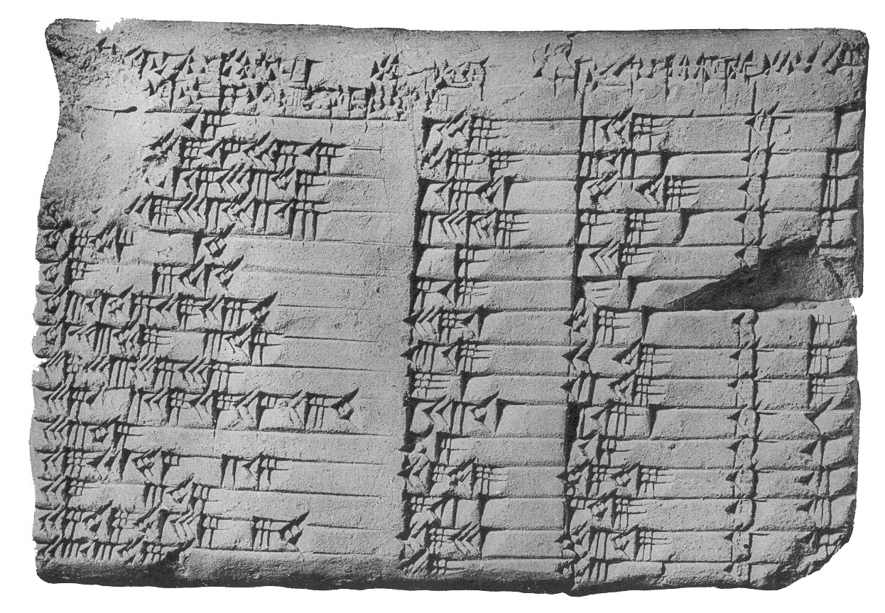
In c. 1800 BCE, a scribe in Larsa (modern day Iraq) wrote a table of numbers on a clay tablet now known as Plimpton 322 (see Figure 1). The second and third columns (from the left) contain pairs \((a, c)\) such that \(c^2 - a^2\) is a square number; for example, on the fourth row we have \(a = 12709\) and \(c = 18541\) and, indeed, \[18541^2 - 12709^2 = 13500^2.\] We can see this as a table of solutions to the Pythagorean equation \[a^2 + b^2 = c^2\] for which \(a, b\) and \(c\) have the nice property of all being integers. Clearly these solutions were not found by trial and error, and this ancient Babylonian had a systematic method of producing them. Later on, Euclid (c. 300 BCE) wrote down formulae which essentially give all integer solutions to this equation.
Proof
If \(a\) and \(b\) are even, then the triple is not primitive. If \(a\) and \(b\) are both odd, then \(a^2 \equiv b^2 \equiv 1 \bmod 4\). Therefore \[c^2 = a^2 + b^2 \equiv 2 \bmod 4.\] As \(2 \mid c^2\), \(2\mid c\). But then \(4 \mid c^2\) and so \(c^2 \equiv 0 \bmod 4\), a contradiction. □
By switching \(a\) and \(b\) if necessary, it is enough to classify primitive triples with \(b\) even. We need one more ingredient, which is where unique factorisation in \(\Z \) comes in.
Proof
We may factorise \begin{align*} x &= \prod _{i=1}^{k} p_i^{a_i}\\ y &= \prod _{j=1}^{l} q_j^{b_j} \end{align*}
where \(p_1, \ldots , p_k\) are distinct primes, \(q_1, \ldots , q_l\) are distinct primes, and all the exponents \(a_i, b_j\) are positive. As \(x\) and \(y\) are coprime, no \(p_i\) is equal to any \(q_j\), and so \[xy = \prod _{i=1}^{k} p_i^{a_i} \prod _{j=1}^{l} q_j^{b_j}\] is the factorisation of \(xy\) into powers of distinct primes. As \(xy\) is a square, the uniqueness of factorisation in \(\Z \) tells us that every \(a_i\) and every \(b_j\) is even. Therefore \(x\) and \(y\) are squares. □
We can now classify primitive Pythagorean triples.
Theorem 1.5. If \((a,b,c)\) is a primitive Pythagorean triple with \(b\) even then there are integers \(m > n > 0\) such that \begin{align*} a &= m^2 - n^2 \\ b &= 2mn \\ c &= m^2 + n^2. \end{align*}
We must have \(m, n\) coprime and of opposite parity, and for every such pair \((m,n)\) these formulae do produce a Pythagorean triple.
Proof
Suppose that \(a, b, c\) is a primitive triple with \(b\) even. Then \[a^2 = c^2 - b^2 = (c-b)(c+b).\] Note that \begin{align*} \gcd (c-b, c+b) &= \gcd (c-b, 2b) \tag *{(as $c + b = (c-b) + 2b$)} \\ &= \gcd (c-b, b) \tag *{(as $c - b$ is odd)} \\ &= \gcd (c,b) \tag *{(as $c = (c-b) + b$)} \\ &= 1 \tag *{(by exercise~\ref {ex:pythag-coprime}).} \end{align*}
By Lemma 1.4, there are positive integers \(r\) and \(s\) with \[c + b = r^2, \qquad c - b = s^2.\] Since \(c \pm b\) are odd, \(r\) and \(s\) are both odd, so \[m = \frac {r + s}{2}, \qquad n = \frac {r - s}{2}\] are integers. Then \begin{align*} m^2 + n^2 &= \frac {r^2 + s^2}{2} = c, \\ 2mn &= \frac {r^2 - s^2}{2} = b, \\ m^2 - n^2 &= rs. \end{align*}
As \(a^2 = (c+b)(c-b) = r^2s^2\), we have \(a = rs = m^2 - n^2\) as required.
We leave the final sentence of the theorem as Exercise 1.6. □
Exercise 1.6. Show that the integers \(m\) and \(n\) in Theorem 1.5 must be coprime and of opposite parity. Conversely, show that if \(m > n > 0\) are coprime integers of opposite parity, then \((m^2 - n^2, 2mn, m^2 + n^2)\) is a primitive Pythagorean triple.
For example, the fourth row of Plimpton 322 is the triple \[(12709, 13500, 18541),\] which comes from \((m, n) = (125, 54)\).
Polynomial equations with integer coefficients, where the task is to find integer (or rational) solutions, are now known as Diophantine equations, after the Greek author Diophantus who lived in Alexandria in around 250 CE. His Arithmetica compiled an extensive list of such equations, together with methods of finding solutions.
Pierre de Fermat, in around 1637, annotated his copy of the Arithmetica (in fact, a Latin translation and commentary by his contemporary Bachet) with the following (in)famous quote:
It is impossible to separate a cube into two cubes, or a fourth power into two fourth powers, or in general any power higher than the second into two like powers. I have discovered a truly marvellous proof of this, which this margin is too narrow to contain.
In other words, for \(n > 2\) a natural number there are no integer solutions to the equation \[a^n + b^n = c^n\] (except for the trivial solutions where one of \(a, b, c\) is zero). Nobody really believes that he had a proof — although he did write down a proof for \(n = 4\) in another marginal note — and the full solution was only found by Andrew Wiles in 1994 using highly advanced methods that Fermat could not have dreamed of (in fact, Wiles’s first solution had an error that he resolved in collaboration with his student Richard Taylor).
Before Wiles, one promising strategy was to copy what we did for \(n = 2\): write \[a^n = c^n - b^n = \prod _{i=0}^{n-1} (c - \zeta _n^i b)\] and try to deduce that the factors on the right hand side must be \(n\)th powers and conclude from there. This requires developing a theory of primality and unique factorisation for numbers in \(\Z [\zeta _n]\), that is, integer linear combinations of \(n\)th roots of unity. Unfortunately, as Kummer realised in 1844, the ring \(\Z [\zeta _n]\) is not always a unique factorisation domain (\(n = 23\) is the first example) and this presents fundamental difficulties for this strategy. Nonetheless, developing number theory in such rings led to a rich theory now known as algebraic number theory, which is the main topic of this module (although our focus will be more on the quadratic rings \(\Z [\sqrt {d}]\)).
In fact, Kummer was probably more motivated by the problem of generalising quadratic reciprocity, a theorem conjectured by Euler in 1783 and proved by Gauss in 1796 that concerns the solvability of congruences such as \(x^2 \equiv a \bmod p\) for \(p\) a prime. We will cover this in detail later this term. To generalise the theory to “higher reciprocity laws”, about the solvability of \(x^n \equiv a \bmod p\), requires arithmetic in \(\Z [\zeta _n]\).
We end with a few other Diophantine equations that algebraic number theory touches upon:
- Which integers \(n\) can be written as sums of two squares? We will answer this one quite soon (Fermat was the first to figure it out). On the other hand, if you want to know which integers (or which primes) can be written as (say) \(x^2 + 14y^2\), the answer becomes rather more complicated and well beyond what we will cover.
- Which integers \(n\) can be written as sums of four squares? All of them (Lagrange)! We won’t prove this, though it can be done in an elementary way. (Why did we miss three squares? It is also interesting, but rather more complicated.)
- Which integers \(n\) can be the area of a right-angled triangle with rational sides? This is the so-called congruent number problem. Fermat (him again...) showed that \(n = 1, 2, 3\) don’t work; in general this belongs to the subject of elliptic curves and a full answer hinges on the (very much open) Birch and Swinnerton–Dyer conjecture.
- For \(d \in \N \), find all solutions to \(x^2 - dy^2 = 1\). This so-called Pell equation was studied by the ancient Greeks and Fermat, and also by Indian mathematicians Brahmagupta (c. 600 CE) and Bhāskara II (c. 1150 CE). We will solve it at the end of term, as an application of the theory of units in \(\Z [\sqrt {d}]\). If 1 is replaced by \(-1\) on the right hand side we know of no simple necessary and sufficient criterion for the equation to have an integer solution.
2 EDs, PIDs and UFDs
2.1 Euclidean domains
Definition 2.1. Let \(R\) be an integral domain. A Euclidean function (or norm) on \(R\) is a function \(\phi :R\setminus \{0\}\rightarrow \N \cup \{0\}\) such that
- For all \(x,y\in R\setminus \{0\}\), we have \(\phi (x)\leq \phi (xy)\),
- For every \(x\in R\) and \(y\in R\setminus \{0\}\), there exist \(q,r\in R\) such that \(x=qy+r\) with either \(r=0\) or \(\phi (r)<\phi (y)\).
If \(R\) has a Euclidean function, then it is called a Euclidean domain (ED).
Another, less obvious, example of an ED is the ring \[\Z [i] = \{a + bi : a, b \in \Z \}\] of Gaussian integers. To show that this is Euclidean we will need the norm \[ N:\Q [i]\longrightarrow \Q ,\qquad N(a+bi)=a^{2}+b^{2}. \] Since \(N(x)=x\bar {x}\) (complex conjugate), we see that \(N\) is multiplicative: \(N(xy)=xy\overline {xy}=x\bar {x}y\bar {y}=N(x)N(y)\). Note that if we restrict the function \(N\) to the subring \(\Z [i]\) of \(\Q [i]\), then its values lie in \(\N \cup \{0\}\) (as \(a^{2}+b^{2}\geq 0\)).
Proof
The first property of a Euclidean function is straightforward: \[N(xy) = N(x)N(y) \ge N(x)\] if \(x, y \in \Z [i]\) are nonzero, since \(N(a + bi) = a^2 + b^2 \ge 1\) for all \(a, b \in \Z \) not both zero.
For the second property, let \(x, y \in \Z [i]\) be nonzero and let \[\lambda = x/y = a + ib\] with \(a, b \in \Q \). Then the key point is that there exists \(q \in \Z [i]\) with \(N(\lambda - q) < 1\). Indeed, let \(a'\) and \(b'\) be (respectively) the closest integers to \(a\) and \(b\) and set \(q = a' + b'i\). Then \[N(\lambda - q) = |(a' - a) + (b'-b)i|^2 =(a'-a)^2 + (b'-b)^2 \le 1/4 + 1/4 < 1.\] Thus \[N(x - qy) = N(y)N(\lambda - q) < N(y)\] and so \(x = qy + r\) with \(r \in \Z [i]\) and \(N(r) < N(y)\). □
We can picture this proof as follows: the ring \(\Z [i]\) sits in the complex plane as the lattice of points with integer coordinates. Every element of \(\C \) may be translated by an element of this lattice to land inside the square \([-1/2, 1/2] \times [-1/2, 1/2]\), which is strictly in the circle of radius 1 (see Figure 2).
![[Picture]](notes0x.svg)
Next, recall the notion of Principal Ideal Domain (PID) from Algebra II (see Section 0.4).
Proof
Let \(R\) be an ED with Euclidean function \(\phi \). Let \(I\) be an ideal of \(R\). If \(I=(0)\), then \(I\) is principal, so we can assume without loss of generality that \(I\) is non-zero. Thus, there exists a non-zero \(x\in I\). Assume that \(x\) is chosen to have minimal Euclidean norm among all non-zero elements of \(I\), that is, \(\phi (x)\leq \phi (y)\) for all non-zero \(y\in I\). (Note that this is possible, as the values of \(\phi \) are natural numbers or zero). We claim that \(I=(x)\). Indeed, let \(y\in I\). Then there exist \(q,r\in R\) such that \[ y=qx+r, \] where \(r=0\) or \(\phi (r)<\phi (x)\). As \(r = y - qx \in I\), the latter inequality is impossible by our choice of \(x\), so we must have \(r=0\) and hence \(y\in (x)\). □
In particular, by the preceding lemma, this shows that \(\Z [i]\) is a PID. However, the converse of the above theorem is false: one can show that \(\Z [\frac {1+\sqrt {-19}}{2}]\) is a PID, but not an ED. The fact that it is a PID will be proved next term.
Remark. (nonexaminable) Note that the proof of Theorem 2.5 did not use the first property of Euclidean norms. Sometimes Euclidean norms are defined to be functions satisfying only the second condition. One can show that if \(R\) is a ring with such a function, then there is always another function on \(R\), namely \(f(a)=\min _{x\in R\setminus \{0\}}\phi (xa)\), that is a Euclidean norm in our sense (that is, \(f\) satisfies both conditions).
2.2 Every PID is a UFD
Example 2.7. For a general integral domain it is not true that every non-zero non-unit element can even be decomposed into a product of irreducible elements (let alone in a unique way). It is a natural reaction to find this counter-intuitive. One of the simplest examples of such a ring is the subring \[ R=\{f(x)\in \Q [x]\mid f(0)\in \Z \} \] of the ring of polynomials \(\Q [x]\) whose constant term is an integer (if it is not clear, check that it is a subring). Note that the only units in \(R\) are \(\pm 1\) (an Algebra II exercise). Thus \(x\) is not irreducible, as (for example) \(x = (x/2)\times 2\) and neither factor is a unit. Suppose that \(x\) can be factored into irreducibles. Then each factor divides \(x\) in \(\Q [x]\), so is either of the form \(cx\), \(c \in \Q \), or of the form \(n\), \(n \in \Z \). But \(cx\) is reducible if \(c \in Q\) for the same reason that \(x\) is reducible, so there are no factors of this form. But then all the factors are constant, but \(x\) is not a constant, which is impossible.
It turns out, however, that “most” rings that we encounter do have decompositions into irreducibles. To get this property, one has to impose some kind of finiteness condition. One such condition is that of Noetherian rings, which we will not cover. But even when we do have decompositions into irreducibles, there may be more than one such decomposition (as the example \(2\cdot 3=(1+\sqrt {-5})(1-\sqrt {-5})\) in \(\Z [\sqrt {-5}]\) shows; see Section 0.2). Factorisation into irreducibles is mostly useful when the ring is a UFD. It is therefore an important result that every PID is a UFD, and this is what we will prove now.
Recall that in an integral domain prime elements are always irreducible (Lemma 0.4). The converse does not always hold, but we do have:
Proof
We already showed in Algebra II that if \(x\) is an irreducible element of a PID then \((x)\) is a maximal ideal (Proposition 0.11). As a maximal ideal is prime (Corollary 0.10), we have that \((x)\) is a prime ideal. It follows that \(x\) is a prime element: certainly \(x\) is nonzero and not a unit (as it is irreducible), and if \(x \mid ab\) then \(ab \in (x)\), so \(a \in (x)\) or \(b \in (x)\) — as \((x)\) is prime — and so \(x \mid a\) or \(x \mid b\) as required. □
Proof
Let \(R\) be a PID. We show that any non-zero non-unit in \(R\) is expressible as a product of irreducibles (and hence as a product of primes), and then show that the factorisation is unique.
Suppose that there is a non-zero non-unit \(a\in R\) that is not the product of irreducibles. Then \(a\) is not irreducible (that is, not the product of one irreducible), so \[ a=bc \] for some non-units \(b,c\in R\). At least one of \(b\) or \(c\) cannot be the product of irreducibles, as otherwise \(a=bc\) would be. Thus \(a\) has a proper factor, say \(a_{1}\), that is not the product of irreducibles and we have an inclusion \[ (a)\subsetneq (a_{1}), \] which is strict (not an equality) as otherwise \(a\) would be a unit times \(a_{1}\), so \(a_{1}\) would not be a proper factor of \(a\). Continuing this argument, we obtain1 an infinite chain of ideals with strict inclusions \[ (a)\subsetneq (a_{1})\subsetneq (a_{2})\subsetneq \cdots . \] But then the union \(\bigcup _{i=1}^\infty (a_i)\) is also an ideal of \(R\) and so is principal, of the form \((a_\infty )\). Then \(a_\infty \in (a_n)\) for some \(n \in \N \) and so \((a_\infty ) \subset (a_i) \subset (a_\infty )\) for all \(i \ge n\). But then \((a_n) = (a_{n+1}) = \ldots \) contradicting that the inclusions above are strict. Thus every non-zero non-unit in \(R\) must be the product of irreducibles.
Uniqueness: (This is the same argument as for \(\Z \) or \(F[x]\) in Algebra II.) Suppose that \[ a=p_{1}p_{2}\cdots p_{n}=q_{1}q_{2}\cdots q_{m}, \] where \(p_{i}\) and \(q_{j}\) are irreducible. By Lemma 2.8, the factors are prime; thus \(p_{1}\mid q_{1}\cdots q_{m}\), so \(p_{1}\) must divide some \(q_{j}\). Reordering if necessary, we can assume that \(j=1\). Then \(p_{1}=u_{1}q_{1}\), for some unit \(u_{1}\in R\) (as \(q_{1}\) is irreducible and \(p_{1}\) is not a unit). Cancelling the factor \(q_{1}\), we get \[ u_{1}p_{2}\cdots p_{n}=q_{2}\cdots q_{m}, \] and continuing this process finitely many times, we obtain:
- if \(n<m\): \(u_{1}\cdots u_{n}=q_{n+1}\cdots q_{m}\); contradiction, as this implies that \(q_{n+1}\) is a unit (while it is irreducible);
- if \(n>m\): \((u_{1}\cdots u_{m})p_{m+1}\cdots p_{n}=1\); contradiction (as before).
Thus \(n=m\) and every \(p_{i}\) on the left-hand side equals some \(q_{j}\) on the right-hand side, up to a unit, proving the uniqueness statement. □
2.3 Application: a Mordell equation
In this section we will apply the theory of Euclidean domains to find all integer solutions to the equation \(y^2 = x^3 - 2\), following a method due to Euler. This particular equation appears already in Diophantus, who observes that \((x,y) = (3,5)\) is a solution. Bachet gave a method to produce new rational solutions from old ones; in this case, his method gives new solutions \[ \left (\frac {129}{10^2}, \pm \frac {383}{10^3}\right ) \quad \text {and}\quad \left (\frac {2340922881}{7660^2}, \pm \frac {113259286337279}{7660^3}\right ). \] Equations of the form \(y^2 = x^3 + n\), \(n \in \Z \) nonzero, are called Mordell equations, after Louis Mordell who proved in 1922 that, for every \(n\), there is a finite number of solutions such that all rational solutions can be generated from them by a method similar to Bachet’s (in fact, he proved this for a more general class of equations known as elliptic curves).
First we require some preliminaries about \(\Z [\sqrt {-2}]\).
Proof
The first part is Exercise 2.4 (1) and Theorems 2.5 and 2.9. The second part is straightforward: if \(x = a + b\sqrt {-2}\) is a unit, then \(xy = 1\) for some \(y \in \Z [\sqrt {-2}]\) and so \(N(x)N(y) = 1\). As \(N(y) \in \N \), \(N(x) = a^2 + 2b^2 = 1\), which is only possible if \(a = \pm 1\) and \(b = 0\). □
Proof
We rewrite the equation as \[y^2 + 2 = x^3\] and then factorise the left-hand side: \[(y + \sqrt {-2})(y - \sqrt {-2}) = x^3.\] We will show that \(y + \sqrt {-2}\) and \(y - \sqrt {-2}\) have no irreducible common factors. Indeed, if \(\pi \) is irreducible and \(\pi \) divides both terms, then \(\pi \) divides their difference \(2\sqrt {-2} = -(\sqrt {-2})^3\). Thus \(\pi = \pm \sqrt {-2}\), as this is irreducible (why?) and \(\Z [\sqrt {-2}]\) is a UFD. But then \(-\pi ^2 = 2 \mid x^3\) in \(\Z [\sqrt {-2}]\), which implies that \(x^3\) is even (why?) and so \(x\) is even. Thus \(y^2 = x^3 - 2\) is even and so \(y\) is even. But then \(y^2 + 2\) is \(2 \bmod 4\) and \(x^3\) is \(0 \bmod 4\), contradiction.
As \(\Z [\sqrt {-2}]\) is a UFD and its units are \(\pm 1\), we may write \[y + \sqrt {-2} = \pm \prod _{i=1}^r \pi _i^{e_i}\] with \(\pi _i\) irreducible elements, \(e_i \in \N \), and \(\pi _i \ne \pm \pi _j\) for \(i \ne j\). Applying complex conjugation to both sides we obtain \[y - \sqrt {-2} = \pm \prod _{i=1}^r \bar {\pi }_i^{e_i}\] and, since they have no common factors, we have \(\pi _i \ne \pm \bar {\pi }_j\) for all \(i, j\). Their product then has factorisation \[\prod _{i=1}^r \pi _i^{e_i}\bar {\pi }_i^{e_i}.\] Considering the factorisation of \(x\) we see that all exponents in the factorisation of \(x^3\) are divisible by 3, and so \(3 \mid e_i\) for all \(i\). In particular, \(y + \sqrt {-2}\) is itself a perfect cube: \[y + \sqrt {-2} = (a + b\sqrt {-2})^3\] for some \(a, b \in \Z \). Comparing coefficients, we obtain \begin{align*} y &= a^3 - 6ab^2 = a(a^2 - 6b^2) \\ 1 &= 3a^2 b - 2b^3 = b(3a^2 - 2b^2). \end{align*}
From the second of these, we see that \(b = 1\) and \(3a^2 - 2 = 1\), or \(b = -1\) and \(3a^2 - 2 = -1\). The first case gives \(a = \pm 1\) and so \(y = \pm 5\), so \(x = 3\), while the second case does not lead to a solution. Thus \(x = 3, y = \pm 5\) is the only solution in integers to the original equation. □
3 Sums of two squares
Fermat, around 1640, determined which integers can be written as a sum of two squares2. The result is:
We will view this as a theorem about factorisation in the UFD \(\Z [i]\). Our first task is to consider the factorisation of (usual) primes \(p\) in \(\Z [i]\). For this we will need to know the units of \(\Z [i]\).
Proposition 3.3. Let \(p \in \Z \) be prime. Then the following are equivalent:
- \(p\) can be written in the form \(a^2 + b^2\) with \(a, b \in \Z \);
- \(p\) is reducible in \(\Z [i]\);
- there is a solution to the congruence \(x^2 \equiv -1 \bmod p\);
- there is a solution to the congruence \(a^2 + b^2 \equiv 0 \bmod p\) with \(a, b \not \equiv 0 \bmod p\).
Proof
We show that (3) implies (2) implies (1) implies (4) implies (3).
(3) implies (2): Suppose that we can solve \(x^2 \equiv -1 \bmod p\). Then we have \[p \mid x^2 + 1 = (x + i)(x - i).\] As \((x \pm i)/p \not \in \Z [i]\), \[p \nmid x \pm i.\] Therefore \(p\) is not a prime element. As \(\Z [i]\) is a PID (Lemma 2.3 and Theorem 2.5), this means that \(p\) is reducible, by Lemma 2.8.
(2) implies (1): Suppose that \(p\) is reducible, so that \(p = \pi \pi '\) with neither \(\pi \) nor \(\pi '\) a unit. The units of \(\Z [i]\) are exactly the elements of norm \(1\) (Exercise 3.2), so \(N(\pi ), N(\pi ') \neq 1\). As \(N(\pi )N(\pi ') = N(p) = p^2\), we must have \(N(\pi ) = p\) and so \(p = a^2 + b^2\).
(1) implies (4): Suppose that \(p = a^2 + b^2\). Certainly \(a^2 + b^2 \equiv 0 \bmod p\). Moreover \(p \nmid a, b\): if \(p \mid a\) then \(p \mid b^2\) and so \(p \mid b\), but then \(p^2 \mid a^2 + b^2 = p\).
(4) implies (3): Suppose that \(a^2 + b^2 \equiv 0 \bmod p\) with \(a, b \not \equiv 0 \bmod p\). Then the residue classes \(\bar {a}\) and \(\bar {b}\) are invertible in \(\F _p\), and we obtain \((\bar {a} \bar {b}^{-1})^2 + \bar {1} = 0\) and so \(x^2 \equiv -1 \bmod p\) for any integer \(x\) with \(\bar {x} = \bar {a}\bar {b}^{-1}\). □
Proof
The case \(p = 2\) is clear, so suppose that \(p\) is odd and that \(x^2 \equiv -1 \bmod p\) has a solution. Then we raise both sides to the power \(\frac {p-1}{2}\): \[x^{p-1} \equiv (x^2)^{\frac {p-1}{2}} \equiv (-1)^{\frac {p-1}{2}}.\] As \(x^2 \equiv -1 \bmod p\), we have \(p \nmid x\), so by Fermat’s little theorem (Theorem 0.18) the left-hand side is \(1 \bmod p\). The right-hand side is \(1\bmod p\) if \(p \equiv 1 \bmod 4\) and \(-1 \bmod p\) if \(p \equiv 3 \bmod 4\). Since \(p\) is odd, \(1 \not \equiv -1 \bmod p\) and so we deduce that \(p \equiv 1 \bmod 4\).
Now suppose that \(p \equiv 1 \bmod 4\). Consider the polynomial \[f(x) = x^{p-1} - \bar {1} \in \F _p[x].\] By Fermat’s little theorem, it has \(\pm \bar {j}\) as roots for \(j = 1, \ldots , \frac {p-1}{2}\). By the factor theorem and the fact that \(\F _p[x]\) is a UFD, \[\prod _{j=1}^{\frac {p-1}{2}} (x + \bar {j})(x - \bar {j}) \mid x^{p-1} - \bar {1}\] and as both sides are monic of the same degree, \[\prod _{j=1}^{\frac {p-1}{2}} (x + \bar {j})(x - \bar {j}) = x^{p-1} - \bar {1}.\] Comparing constant terms, we see that \[(-1)^{(p-1)/2}\left (\left (\frac {p-1}{2}\right )!\right )^2 \equiv -1 \bmod p.\] As \(p \equiv 1 \bmod 4\), the initial sign is \(+1\) and so \(x = \left (\frac {p-1}{2}\right )!\) is a solution to \(x^2 \equiv -1 \bmod p\). □
Example 3.5. The primes 5 and 97 are both \(1 \bmod 4\) and indeed \[5 = 1^2 + 2^2 = (1+2i)(1-2i) = N(1 + 2i)\] while \[97 = 4^2 + 9^2 = (4+9i)(4-9i) = N(4 + 9i).\] This gives us two different ways of writing their product as a sum of squares: \[485 = 5 \cdot 97 = N((1+2i)(4 + 9i)) = N(-14 + 17i) = 14^2 + 17^2\] and \[485 = N((1-2i)(4+9i)) = N(22 + i) = 22^2 + 1^2.\]
Proof
(of Theorem 3.1) Suppose first that \(n = a^2 + b^2\). Let \(d\) be the highest common factor of \(a\) and \(b\). Then writing \(a = da'\) and \(b = db'\), we see that \(d^2 \mid n\) and we may write \(n = d^2n'\) with \[n' = (a')^2 + (b')^2\] and \(a'\), \(b'\) coprime. We will show that \(n'\) has no prime factor \(\equiv 3 \bmod 4\). Indeed, suppose that \(p \equiv 3 \bmod 4\) and \(p \mid n'\), so that \((a')^2 + (b')^2 \equiv 0 \bmod p\). If \(p \mid a'\) then \(p \mid (b')^2\) and so \(p \mid b'\), contradicting that \(a'\) and \(b'\) are coprime; so \(p \nmid a'\), and similarly \(p \nmid b'\). By the implication (4) implies (3) of Proposition 3.3, there is a solution to \(x^2 \equiv -1 \bmod p\). This contradicts Lemma 3.4, as \(p \equiv 3 \bmod 4\). Finally, \(n = d^2n'\), so the squarefree part \(m\) of \(n\) is also the squarefree part of \(n'\). In particular \(m \mid n'\), so \(m\) has no prime factor \(\equiv 3 \bmod 4\) either.
For the other direction, suppose that \(n = t^2m\) and that \(m = p_1\ldots p_r\) with \(p_i \not \equiv 3 \bmod 4\) for all \(i\). Then by Theorem 3.6, there are \(\pi _i \in \Z [i]\) with \(N(\pi _i) = p_i\). Writing \(\pi = \pi _1\ldots \pi _r\), we have \[m = p_1\ldots p_r = N(\pi _1)\ldots N(\pi _r) = N(\pi ).\] Putting \(\pi = a + ib\) we see that \[m = a^2 + b^2\] and so \(n = (ta)^2 + (tb)^2\), as required. □
We can go further and ask whether the expression of \(p\) as a sum of two squares is unique. And indeed:
Proof
Suppose that \(p = a^2 + b^2 = c^2 + d^2\). Then \[(a+ bi)(a - bi) = (c + di)(c - di)\] and all four brackets have prime norm \(p\) and are hence irreducible. By unique factorisation in \(\Z [i]\), \[a + bi = u(c \pm di)\] for some unit \(u \in \Z [i]\). As the only units are \(\pm 1\) and \(\pm i\) (Exercise 3.2), we obtain \[a = \pm c, b = \pm d\] or \[a = \pm d, b = \pm c\] as required. □
4 Finite field extensions
If \(L/F\) is a field extension, then \(L\) is a vector space over \(F\) (it contains \(0\), is closed under addition, and is closed under multiplication by ‘scalars’ i.e. elements of \(F\)).
Example 4.2. \(\Q (\sqrt {-2})\) is isomorphic, as a vector space, to \(\Q ^{2}\), so is a \(2\)-dimensional vector space over \(\Q \). An isomorphism is given by \[ a+b\sqrt {-2}\longleftrightarrow \begin {pmatrix}a\\ b \end {pmatrix} \] so the standard basis \(\left \{ \begin {pmatrix}1\\ 0 \end {pmatrix},\begin {pmatrix}0\\ 1 \end {pmatrix}\right \} \) in \(\Q ^{2}\) corresponds to the basis \(\{1,\sqrt {-2}\}\) in \(\Q (\sqrt {-2})\).
Example 4.6. The element \(i\in \C \) is algebraic over \(\R \) since \(i\) is a root of \(f(x)=x^{2}+1\in \R [x]\). Actually, \(\C \) is algebraic over \(\R \) since any \(z=a+bi\in \C \) is a root of \(f(x)=(x-z)(x-\bar {z})=x^{2}-2ax+a^{2}+b^{2}\).
As transcendental numbers exist (\(\pi \) and \(e\) are examples), \(\R \) is not algebraic over \(\Q \) (and hence not finite, by the following proposition).
Proof
Let \(\alpha \in L\). The elements \(1,\alpha ,\alpha ^{2},\dots ,\alpha ^{[L:F]}\) must be linearly dependent, as there are \([L:F]+1\) of them and \(\dim _{F}L=[L:F]\). This means that there are some \(a_{i}\in F\), not all zero, and \(n\geq 0\) such that \(\sum ^{n}_{i=0}a_{i}\alpha ^{i}=0\), that is, \(\alpha \) is a root of the non-zero polynomial \(f(x)=\sum ^{n}_{i=0}a_{i}x^{i}\). We have shown that an arbitrary \(\alpha \in L\) is algebraic; thus \(L/F\) is algebraic. □
Note that the converse of the above result is not true: there exist algebraic extensions that are infinite, for example the field \(\bar {\Q }\) of all algebraic numbers (more on this later).
4.1 Minimal polynomials
Definition 4.8. Let \(L/F\) be a field extension and \(\alpha \in L\) be algebraic over \(F\). The minimal polynomial of \(\alpha \) (over \(F\)) is the unique monic polynomial \(p_{\alpha , F}(x) \in F[x]\) of minimal degree such that \(p_{\alpha , F}(\alpha ) = 0\). The degree of \(\alpha \) over \(F\) is the degree of \(p_{\alpha , F}\).
Note that, as \(\alpha \) is algebraic, it is a root of some polynomial over \(F\), so the minimal polynomial exists. If \(f(x)\) is another monic polynomial of the same degree such that \(f(\alpha ) = 0\), then \(p_{\alpha , F} - f\) has smaller degree (as both are monic) and still has \(\alpha \) as a root, so must be zero. Thus \(f(x) = p_{\alpha , F}(x)\), which justifies the word ‘unique’ in the definition. When the field \(F\) is understood, we simply write \(p_\alpha = p_{\alpha , F}\).
Proposition 4.9. Let \(L/F\) and \(\alpha \) be as above and let \(f(x) \in F[x]\) be a monic polynomial with \(f(\alpha ) = 0\). The following are equivalent:
- \(f(x)\) is the minimal polynomial of \(\alpha \);
- \(f(x)\) is irreducible;
- \(f(x)\) generates the ideal \[I_\alpha = \{g(x) \in F[x] : g(\alpha ) = 0\}.\]
Proof
(1) implies (2): suppose that \(f(x)\) is the minimal polynomial of \(\alpha \) over \(F\) and that it is reducible. Then \(f(x) = g(x)h(x)\) with \(g(x)\) and \(h(x)\) monic polynomials and \(\deg g, \deg h < \deg f\). As \(f(\alpha ) = 0\), either \(g(\alpha ) = 0\) or \(h(\alpha ) = 0\). Either way, this contradicts the minimality of \(\deg f\).
(2) implies (3): Suppose that \(f(x)\) is irreducible. As \(F[x]\) is a PID, \(I_\alpha = (g(x))\) for some polynomial \(g(x)\) that we may take to be monic. As \(f(\alpha ) = 0\), \(f(x) \in I_\alpha \), and so \(f(x) = g(x)h(x)\) for some \(h(x) \in F[x]\). But \(f(x)\) is irreducible, and \(g(x)\) is nonconstant as \(g(\alpha ) = 0\), so \(h(x) = 1\) and \(f(x) = g(x)\).
(3) implies (1): Suppose that \(I_\alpha = (f(x))\) and that \(g(x)\) is another monic polynomial with \(g(\alpha ) = 0\). Then \(g(x) \in I_\alpha \) and so \(g(x) = f(x) h(x) \) for some (nonzero) \(h(x) \in F[x]\). Thus \(\deg g \ge \deg f\), so \(\deg f\) is minimal among monic polynomials with \(\alpha \) as a root. □
- For \(i\in \C \), we have \(p_{i,\R }(x)=p_{i,\Q }(x)=x^{2}+1\), but \(p_{i,\Q (i)}(x)=x-i\).
- Let \(\alpha =\sqrt [7]{5}\). We claim that \(f(x)=x^{7}-5\) is the minimal polynomial of \(\alpha \). Clearly \(f(\alpha )=0\) so by Proposition 4.9, it is enough to show that \(f(x)\) is irreducible. For this, use Eisenstein’s criterion from Algebra II.
- Let \(\alpha =e^{2\pi i/p}\in \C \), where \(p\) is a prime number. As \(\alpha \) is a root of \(x^p - 1\), it is algebraic. What is its minimal polynomial \(p_{\alpha }(x)\) over \(\Q \)? It cannot be \(x^{p}-1\), as \[ x^{p}-1=(x-1)(x^{p-1}+x^{p-2}+\dots +1) \] is reducible. Let \(\Phi (x)=(x^{p}-1)/(x-1)\) be the second factor. We must have \(\Phi (\alpha )=0\), as \(\alpha \neq 1\). We claim that \(\Phi (x)\) is irreducible and hence that \(p_{\alpha }(x)=\Phi (x)\). To show this, apply Eisenstein’s criterion to \[ \Phi (x+1)=x^{p-1}+\binom {p}{1}x^{p-2}+\dots +p, \] using the fact that \(p\) divides all the binomial coefficients \(\binom {p}{j}\) for \(1\leq j\leq p-1\). If \(\Phi (x)\) were reducible, we would have \(\Phi (x)=g(x)h(x)\), for some \(g(x),h(x)\) of degree less than \(\deg \Phi \). Hence \(\Phi (x+1)=g(x+1)h(x+1)\), which we have just shown is impossible.
4.2 Fields generated by elements
Let \(L/F\) be a field extension and let \(\alpha \in L\) (not necessarily algebraic over \(F\)). We define \(F(\alpha )\subset L\) to be the smallest field extension of \(F\) that contains \(\alpha \); we call \(F(\alpha )\) the field generated by \(\alpha \) over \(F\) or “\(F\) adjoin \(\alpha \)”. We can describe it quite explicitly: \[F(\alpha ) = \left \lbrace \frac {p(\alpha )}{q(\alpha )} : p(x), q(x) \in F[x], q(\alpha ) \ne 0\right \rbrace .\] Indeed, it is easy to check that the right hand side is indeed a field and that it is contained in any subfield of \(L\) that contains \(F\) and \(\alpha \).
More generally, given \(\alpha _{1},\dots ,\alpha _{n}\in L\), we define \(F(\alpha _{1},\dots ,\alpha _{n})\) to be the smallest field extension of \(F\) containing \(\alpha _{1},\dots ,\alpha _{n}\). It has the same description as above, but with \(p(x)\) and \(q(x)\) replaced by polynomials in \(F[x_1, \ldots , x_n]\). In fact, we have \[ F(\alpha _{1},\dots ,\alpha _{n})=F(\alpha _{1},\dots ,\alpha _{n-1})(\alpha _{n})=\dots =F(\alpha _{1})(\alpha _{2})\dots (\alpha _{n}). \] Working inductively, it is enough to show this for two elements: \(F(\alpha ,\beta )=F(\alpha )(\beta )\). Indeed, \(F(\alpha )(\beta )\) contains \(\alpha \) and \(\beta \), so by the minimality of \(F(\alpha ,\beta )\), we have \(F(\alpha ,\beta )\subset F(\alpha )(\beta )\). On the other hand, \(F(\alpha ,\beta )\) contains \(F\) and \(\alpha \), hence it contains \(F(\alpha )\), and since it also contains \(\beta \), the minimality of \(F(\alpha )(\beta )\) implies that \(F(\alpha )(\beta )\subset F(\alpha ,\beta )\).
Warning: Don’t confuse \(F(\alpha )\) with \(F[\alpha ]\). The latter is by definition the ring consisting of polynomials in \(\alpha \), that is, \[ F[\alpha ]=\Big \{\sum ^{n}_{i=0}a_{i}\alpha ^{i}\;\Big |\; a_{i}\in F,\ n\geq 0\Big \}=\{f(\alpha )\mid f(x)\in F[x]\}. \] In general, we have \(F(\alpha )\neq F[\alpha ]\). For example, if \(\alpha \in \C \) is transcendental (that is, not algebraic over \(\Q \)), then \(\Q (\alpha )\neq \Q [\alpha ]\). Indeed, \(\alpha ^{-1}\in \Q (\alpha )\) but \(\alpha ^{-1}\not \in \Q [\alpha ]\), because otherwise we would have \(f(\alpha )=\alpha ^{-1}\) for some polynomial \(f(x)=\sum ^{n}_{i=0}a_{i}x^{i}\in \Q [x]\). But then \(\alpha f(\alpha )=1\), so \(\alpha \) would be a root of the non-zero polynomial \(xf(x)-1\); contradiction, as \(\alpha \) is transcendental.
On the other hand, we do have equality when \(\alpha \) is algebraic.
Lemma 4.11. Let \(L/F\) be a field extension and let \(\alpha \in L\) be algebraic over \(F\) with minimal polynomial \(p_\alpha (x)\).
-
The map \begin{align*}\ev _\alpha : F[x] & \to F[\alpha ]\\ f(x) &\mapsto f(\alpha )\end{align*}
is a surjective \(F\)-linear ring homomorphism with kernel \((p_\alpha (x))\). (This map is called the ‘evaluation map’.)
- \(F[\alpha ]\) is a field and hence \(F[\alpha ] = F(\alpha )\).
Proof
(1). It is clear that \(\ev _\alpha \) is a surjective \(F\)-linear ring homomorphism (for example, \(f(x) + g(x)\) is sent to \(f(\alpha ) + g(\alpha )\), so it is additive). The kernel is \[\{f(x) \in F[x] : f(\alpha ) = 0\}\] which we have already shown (Proposition 4.9) is generated by \(p_\alpha (x)\).
(2). Since \(p_\alpha (x)\) is irreducible and \(F[x]\) is a PID, \((p_\alpha (x))\) is maximal and so \(F[x]/(p_\alpha (x))\) is a field. By the isomorphism theorem for ring homomorphisms, \[F[\alpha ] \cong F[x]/\ker (\ev _\alpha ) = F[x]/(p_\alpha (x)).\] Thus \(F[\alpha ]\) is a field, and so \(F[\alpha ] = F(\alpha )\). □
If \(\alpha \) is algebraic over \(F\), there is a simple relationship between the degree of a field extension \(F(\alpha )/F\) and the degree of \(\alpha \) (if this wasn’t so, it would be very bad to use the same word “degree”):
Proof
Let \(d = \deg p_\alpha \). We show that \(\{1, \alpha , \ldots , \alpha ^{d-1}\}\) is a basis of \(F(\alpha )\) over \(F\).
It spans: by Lemma 4.11, \(F(\alpha ) = F[\alpha ]\), so every element of \(F(\alpha )\) is of the form \(f(\alpha )\) for some \(f(x) \in F[x]\). By Euclid we may write \(f(x) = q(x)p_\alpha (x) + r(x)\) with \(\deg r < d\). Then \(f(\alpha ) = r(\alpha )\), which is in the span of \(\{1, \alpha , \ldots , \alpha ^{d-1}\}\).
It is linearly independent: if \(\sum _{i=0}^{d-1} a_i \alpha ^i = 0\), then \(\alpha \) is a root of \(\sum _{i=0}^{d-1} a_i x^i\), a polynomial of degree less than \(d\). By the minimality of \(\deg p_\alpha \), this polynomial is zero, that is, \(a_i = 0\) for all \(i\). □
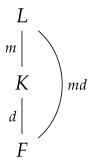
If \(K/F\) and \(L/K\) are field extensions, that is, \(F\subset K\subset L\), then we call this a tower of fields.
The Tower Theorem can be summarised by the following diagram, in which each line is labelled by the degree of the extension.
Proof
We treat the case where \([L:K]\) and \([K:F]\) are finite; the infinite cases are similar. Let \(\{e_{1},\dots ,e_{m}\}\) be a \(K\)-basis of \(L\), where \(m=[L:K]\) and \(\{f_{1},\dots ,f_{d}\}\) an \(F\)-basis of \(K\), where \(d=[K:F]\). We claim that the \(md\) elements \(e_{i}f_{j}\), for \(1\leq i\leq m\) and \(1\leq j\leq d\), form an \(F\)-basis of \(L\).
For any \(\alpha \in L\), we can write \[ \alpha =\sum ^{m}_{i=1}a_{i}e_{i},\qquad a_{i}\in K. \] Moreover, for each \(a_{i}\), we can write \(a_{i}=\sum ^{d}_{j=1}b_{ij}f_{j}\), for some \(b_{ij}\in F\), so that \[ \alpha =\sum ^{m}_{i=1}\sum ^{d}_{j=1}b_{ij}f_{j}e_{i}. \] Thus the \(e_{i}f_{j}\) span \(L\) over \(F\). To show that they are linearly independent, suppose that \[ \sum ^{m}_{i=1}\sum ^{d}_{j=1}c_{ij}e_{i}f_{j}=0, \] for some \(c_{ij}\in F\). Then, as the \(e_{i}\) are linearly independent over \(K\), we must have \[ \sum ^{d}_{j=1}c_{ij}f_{j}=0\qquad \text {for all }i=1,\dots ,m. \] But as the \(f_{j}\) are linearly independent over \(F\), this implies that \(c_{ij}=0\) for all \(i\) and \(j\). □
Example 4.14. Let \(L=\Q (\sqrt {2},\sqrt {3})\). We will show that \([L:\Q ]=4\). Set \(K=\Q (\sqrt {2})\). Then \(L = K(\sqrt {3})\) and \([K:\Q ] = 2\) as \(x^2 - 2\) is irreducible over \(\Q \).
We claim that \(x^{2}-3\) is irreducible over \(K\). Indeed, if not, then \(\sqrt {3}\in K\) so \(\sqrt {3}=a+b\sqrt {2}\) for some \(a,b\in \Q \). But this is impossible: if \(a=0\), then \(\sqrt {6}=2b\in \Q \), contradiction; if \(b=0\), then \(\sqrt {3}\in \Q \), contradiction; if \(a\neq 0\) and \(b\neq 0\), then after squaring, \(3=a^{2}+2b^{2}+2ab\sqrt {2}\), so \(\sqrt {2}\in \Q \), contradiction.
Thus \([L : K] = 2\) and, by the Tower Theorem, we obtain \[ [L:\Q ]=[L:K]\cdot [K:\Q ]=2\cdot 2=4. \]
4.3 Norm and trace
Let \(L/F\) be a finite field extension and \(n=[L:F]\). As usual, we view \(L\) as a vector space over \(F\). Write \(\End _{F}(L)\) for the (noncommutative) ring of \(F\)-linear maps \(L\to L\), with composition as multiplication; it is also a vector space over \(F\). For any \(\alpha \in L\), we have an \(F\)-linear map \[ \hat {\alpha }:L\longrightarrow L,\qquad x\longmapsto \alpha x. \]
Proof
To show that \(\alpha \mapsto \hat {\alpha }\) is an \(F\)-linear ring homomorphism, we must check that, for \(\alpha ,\beta \in L\) and \(c\in F\):
- \(\hat {1}=\Id _{L}\);
- \(\widehat {\alpha +\beta }=\hat {\alpha }+\hat {\beta }\);
- \(\widehat {c\alpha }=c\hat {\alpha }\);
- \(\widehat {\alpha \beta }=\hat {\alpha }\circ \hat {\beta }\).
This is straightforward: for exmaple, \[\widehat {\alpha + \beta }(x) = (\alpha + \beta )x = \alpha x + \beta x = \widehat {\alpha }(x) + \widehat {\beta }(x).\]
Finally, the kernel of the map is \((0)\): if \(\hat {\alpha }=0\) then \(\alpha =\hat {\alpha }(1)=0\). Therefore it is injective. □
Now fix a basis \(\{\alpha _{i}\}_{i=1,\dots ,n}\) of \(L\) over \(F\). Recall from Linear Algebra I that sending an \(F\)-linear map to its matrix with respect to this basis is an isomorphism \(\End _{F}(L)\to \M _{n}(F)\) of rings (and of \(F\)-vector spaces)3. We write \(T_{\alpha }=T_{\alpha ,L/F}\in \M _{n}(F)\) for the matrix of \(\hat {\alpha }\) with respect to our fixed bassi. Spelling out what this means, we have \(T_{\alpha }=(a_{ij})\), where the \(a_{ij}\in F\) are uniquely determined by \begin{align*} \hat {\alpha }(\alpha _{1}) & =\alpha \alpha _{1}=a_{11}\alpha _{1}+\dots +a_{n1}\alpha _{n},\\ \hat {\alpha }(\alpha _{2}) & =\alpha \alpha _{2}=a_{12}\alpha _{1}+\dots +a_{n2}\alpha _{n},\\ & \dots \\ \hat {\alpha }(\alpha _{n}) & =\alpha \alpha _{n}=a_{1n}\alpha _{1}+\dots +a_{nn}\alpha _{n}. \end{align*}
Thus the \(j\)th column of \(T_{\alpha }\) records the ‘coordinates’ of \(\alpha \alpha _{j}\) in the basis \(\{\alpha _1, \ldots , \alpha _n\}\).
Of course, the matrix \(T_{\alpha }\) depends on the choice of basis, but its determinant and trace do not depend on the basis (\(\det (PT_{\alpha }P^{-1})=\det (P)\det (T_{\alpha })\det (P)^{-1}=\det (T_{\alpha })\) and \(\Tr (PT_{\alpha }P^{-1})=\Tr (T_{\alpha }P^{-1}P)=\Tr (T_{\alpha })\); see Linear Algebra I), but only on the linear map \(\hat {\alpha }\), hence only on \(\alpha \). Thus the norm and trace are well-defined.
Example 4.17. Let \(L=\Q (\sqrt {m})\) for \(m\in \Z \) not a square. Take any \(\alpha =a+b\sqrt {m}\in L\). We compute \(N_{L/\Q }(\alpha )\) and \(\Tr _{L/\Q }(\alpha )\). Fix the basis \(\{1,\sqrt {m}\}\) of \(L\) over \(\Q \) and write \begin{align*} \alpha \cdot 1 & =a+b\sqrt {m},\\ \alpha \sqrt {m} & =bm+a\sqrt {m}, \end{align*}
so that \[ T_{\alpha }=\begin {pmatrix}a & bm\\ b & a \end {pmatrix} \] and therefore \[ N_{L/\Q }(\alpha )=a^{2}-mb^{2}\qquad \text {and}\qquad \Tr _{L/\Q }(\alpha )=2a. \]
The following lemma will be used several times in the following in the computation of norms and traces.
Proof
The map \(\alpha \mapsto T_{\alpha }\) is the composition of the map of Lemma 4.15 with the isomorphism \(\End _{F}(L)\to \M _{n}(F)\), so it is an injective \(F\)-linear ring homomorphism. For the last assertion, write \(f(x)=a_{0}+a_{1}x+\dots +a_{k}x^{k}\), \(a_{i}\in F\) and use additivity, \(F\)-linearity and multiplicativity: \[ T_{f(\alpha )}=\sum ^{k}_{i=0}T_{a_{i}\alpha ^{i}}=\sum ^{k}_{i=0}a_{i}T_{\alpha ^{i}}=\sum ^{k}_{i=0}a_{i}T^{i}_{\alpha }=f(T_{\alpha }). \] □
This lemma says that if we want to compute, for example, \(N_{L/F}(\alpha ^{3}+1)\), then we can either compute \(\det (T_{\alpha ^{3}+1})\) or first compute \(T_{\alpha }\) and then take the \(\det (T^{3}_{\alpha }+I)\), where \(I\) is the identity matrix. Usually the former method involves fewer calculations, but for theoretical reasons, as we will soon see, it is important to know that both lead to the same answer.
We now state some basic properties of the norm and trace.
Proposition 4.19. Let \(L/F\) be as above. Then, for all \(\alpha ,\beta \in L\), we have
- \(N_{L/F}(\alpha )=0\) if and only if \(\alpha =0\),
- \(N_{L/F}(\alpha \beta )=N_{L/F}(\alpha )N_{L/F}(\beta )\),
- for \(a\in F\), we have \(N_{L/F}(a)=a^{[L:F]}\) and \(\Tr _{L/F}(a)=[L:F]a\),
- for all \(a,b\in F\), we have \[ \Tr _{L/F}(a\alpha +b\beta )=a\Tr _{L/F}(\alpha )+b\Tr _{L/F}(\beta ), \] that is, \(\Tr _{L/F}\) is an \(F\)-linear map.
Proof
- The map \(\hat {\alpha }\), and hence the matrix \(T_{\alpha }\), is invertible if \(\alpha \neq 0\) (as the inverse is then \(\widehat {\alpha ^{-1}}\)). Thus \(\det (T_{\alpha })=0\) if and only if \(\alpha =0\).
- Follows from the multiplicativity of the determinant.
- For \(a\in F\), we have \(T_{a}=aI\), where \(I\) is the identity matrix of size \([L:F]\).
- Follows from \(T_{a\alpha +b\beta }=aT_{\alpha }+bT_{\beta }\) (Lemma 4.18) and the fact that the trace of a matrix is the sum of the diagonal entries.
4.4 Characteristic polynomials
Let \(A\in \M _{n}(F)\) be a matrix and recall from Linear Algebra I that the characteristic polynomial \(\chi _{A}(x)\) of \(A\) is \[ \det (xI-A)\in F[x]. \] The polynomial \(\chi _{A}(x)\) is monic of degree \(n\). It is a fact from Linear Algebra that if \(\chi _{A}(x)=x^{n}+c_{n-1}x^{n-1}+\dots +c_{0}\), then \[ \det (A)=(-1)^{n}c_{0}\qquad \text {and}\qquad \Tr (A)=-c_{n-1}. \] To see this, let \(\alpha _{1},\dots ,\alpha _{n}\) be the eigenvalues of \(A\) (in some field extension \(L\) of \(F\) that contains all the eigenvalues, for example \(L=F(\alpha _{1},\dots ,\alpha _{n})\)). Then \(\det (A)=\alpha _{1}\cdots \alpha _{n}\) and \(\Tr (A)=\alpha _{1}+\dots +\alpha _{n}\) (because there exists a \(g\in \GL _{n}(L)\) such that \(gAg^{-1}\) is upper triangular, hence with its eigenvalues on the diagonal, by triangularising over a splitting field), while \[ \chi _{A}(x)=(x-\alpha _{1})\cdots (x-\alpha _{n})=x^{n}-(\alpha _{1}+\dots +\alpha _{n})x^{n-1}+\cdots +(-1)^{n}(\alpha _{1}\cdots \alpha _{n}). \]
Now, if \(L/F\), \(n=[L:F]\), is a finite extension and \(\alpha \in L\), then we have the matrix \(T_{\alpha ,L/F}\in \M _{n}(F)\) (depending on a choice of \(F\)-basis for \(L\)) and we denote its characteristic polynomial \(\chi _{\alpha }=\chi _{\alpha ,L/F}\) (this does not depend on the choice of basis, as \(\det (xI-P^{-1}AP)=\det (xI-A)\)). From the above discussion about \(\det \) and \(\Tr \) it follows that if we write \(\chi _{\alpha }(x)=x^{n}+c_{n-1}x^{n-1}+\dots +c_{0}\), \(c_{i}\in F\), then \begin{equation} N_{L/F}(\alpha )=(-1)^{n}c_{0}=\alpha _{1}\cdots \alpha _{n}\qquad \text {and}\qquad \Tr _{L/F}(\alpha )=-c_{n-1}=\alpha _{1}+\dots +\alpha _{n}, \tag{1}\end{equation} where the \(\alpha _{i}\) are the eigenvalues of \(T_{\alpha ,L/F}\), that is, the roots of \(\chi _{\alpha }(x)\).
By the Cayley–Hamilton theorem, \(\chi _{\alpha }(T_{\alpha })=0\), so by Lemma 4.18, \(T_{\chi _{\alpha }(\alpha )}=\chi _{\alpha }(T_{\alpha })=0\). By the injectivity in Lemma 4.18, \(\chi _{\alpha }(\alpha )=0\), so \(\chi _{\alpha }(x)\) has \(\alpha \) as a root, just like the minimal polynomial \(p_{\alpha }(x)\) of \(\alpha \) over \(F\). What is the relation Lecture 11between \(\chi _{\alpha }\) and \(p_{\alpha }(x)\)? When \(\alpha \) generates \(L\) the answer is easy:
Proof
We have already seen that \(\chi _{\alpha }(x)\) is monic of degree \([L:F]\) and \(\chi _{\alpha }(\alpha )=0\). By Lemma 4.12, \[ \deg p_{\alpha }(x)=[L:F]=\deg \chi _{\alpha }, \] so by the uniqueness of the minimal polynomial (Proposition 4.9 (1)), we have \(\chi _{\alpha }(x)=p_{\alpha }(x)\). □
When \(\alpha \in L\) doesn’t generate \(L\) over \(F\), we can still determine \(\chi _{\alpha }(x)\) in terms of \(p_{\alpha }(x)\). As before, let \(n=[L:F]\) and \(d=[F(\alpha ):F]\). Also put \(m:=n/d=[L:F(\alpha )]\) (by the Tower Theorem). To help to keep track of what is going on, we recall the diagram we saw earlier in connection with the Tower Theorem, now applied to the tower \(F\subset F(\alpha )\subset L\):
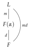
Proposition 4.21. Let \(L/F\) and \(\alpha \in L\) be as above, with \(p_{\alpha }(x)=x^{d}+a_{d-1}x^{d-1}+\dots +a_{0}\), \(a_{i}\in F\), and let \(m=[L:F(\alpha )]\). Then
- \(\chi _{\alpha }(x)=p_{\alpha }(x)^{m}\);
- \(N_{L/F}(\alpha )=N_{F(\alpha )/F}(\alpha )^{m}=(-1)^{md}a^{m}_{0}\);
- \(\Tr _{L/F}(\alpha )=m\Tr _{F(\alpha )/F}(\alpha )=-ma_{d-1}\).
Proof
(1): Let \(\alpha _{1},\dots ,\alpha _{d}\) be an \(F\)-basis of \(F(\alpha )\) (for example, the basis \(1,\alpha ,\dots ,\alpha ^{d-1}\)) and let \(\beta _{1},\dots ,\beta _{m}\) be an \(F(\alpha )\)-basis of \(L\). Then, by the proof of the Tower Theorem, an \(F\)-basis of \(L\) is \[ \{\alpha _{1}\beta _{1},\dots ,\alpha _{d}\beta _{1},\dots ,\alpha _{1}\beta _{m},\dots ,\alpha _{d}\beta _{m}\}. \] Since \(\alpha \in F(\alpha )\), for \(1\leq i,j\leq d\) there are \(c_{ij}\in F\) such that \(\alpha \alpha _{j}=\sum ^{d}_{i=1}c_{ij}\alpha _{i}\); thus \[ T_{\alpha ,F(\alpha )/F}=(c_{ij})_{ij}\in \M _{d}(F). \] Since \(\alpha \cdot \alpha _{j}\beta _{k}=\sum ^{d}_{i=1}c_{ij}\alpha _{i}\beta _{k}\) (and the \(\alpha _{i}\beta _{k}\) form an \(F\)-basis of \(L\)), we have that \(T_{\alpha ,L/F}\) is a block diagonal matrix with \(m\) repeated \(d\times d\) blocks equal to \(T_{\alpha ,F(\alpha )/F}\), that is, \[ T_{\alpha ,L/F}=\begin {pmatrix}T_{\alpha ,F(\alpha )/F} & & 0\\ & \ddots \\ 0 & & T_{\alpha ,F(\alpha )/F} \end {pmatrix}. \] Since the determinant of a block diagonal matrix is the product of the determinants of the blocks, we get \[ \chi _{\alpha }(x)=\chi _{\alpha ,L/F}(x)=\det (xI-T_{\alpha ,L/F})=\det (xI-T_{\alpha ,F(\alpha )/F})^{m}=\chi _{\alpha ,F(\alpha )/F}(x)^{m}=p_{\alpha }(x)^{m}, \] where the last equality is by Lemma 4.20.
(2) and (3): The first equalities follow from considering the determinant and trace of the block matrix above. The second equalities then follow from \(N_{F(\alpha )/F}(\alpha )=(-1)^{d}a_{0}\) and \(\Tr _{F(\alpha )/F}(\alpha )=-a_{d-1}\), which hold by Lemma 4.20 and equation (1). □
It’s natural to ask what happens to norms and traces in a tower: if \(L/K/F\) are finite field extensions and \(\alpha \in L\), how are \(N_{L/K}(\alpha )\) and \(N_{L/F}(\alpha )\) related (and similarly for traces)? The answer is simple and easy to remember, but unfortunately the proof is rather involved and nonexaminable. If you are studying Galois theory, then a simpler proof can be given using ideas from that course.
Proof sketch (nonexaminable)
We can quickly reduce to the case \(L = K(\alpha )\) using Proposition 4.21 (2) and (3). (In fact, Proposition 4.21 parts (2) and (3) follow from Theorem 4.22, but our proof depends on having proved those consequences first.)
So suppose that \(L=K(\alpha )\), let \(n=[K:F]\) and \(d=[L:K]\), and let \[ p_{\alpha ,K}(x)=x^{d}+a_{d-1}x^{d-1}+\dots +a_{0},\qquad a_{i}\in K. \] Let \(\beta _1, \ldots , \beta _n\) be a basis for \(K/F\). By the proof of the Tower Theorem, an \(F\)-basis for \(L\) is \[ \beta _1, \ldots , \beta _n,\ \alpha \beta _1, \ldots , \alpha \beta _n, \ldots ,\alpha ^{d-1}\beta _1, \ldots , \alpha ^{d-1}\beta _n. \] We compute \(T_{\alpha ,L/F}\) in this basis, as a \(d\times d\) matrix of \(n\times n\) blocks. For \(j<d-1\), multiplication by \(\alpha \) sends \(\alpha ^{j}\beta _i\) to \(\alpha ^{j+1}\beta _i\), while \[ \alpha \cdot \alpha ^{d-1}\beta _i=\alpha ^{d}\beta _i=-\sum _{j=0}^{d-1}\alpha ^{j}(a_j\beta _i), \] and the coordinates of \(a_j\beta _i\) with respect to \(\beta _1,\ldots ,\beta _n\) form the \(i\)th column of \(A_j=T_{a_j,K/F}\). Hence \[ T_{\alpha ,L/F}=\begin {pmatrix} 0 & 0 & \cdots & 0 & -A_{0}\\ I & 0 & \cdots & 0 & -A_{1}\\ 0 & I & \cdots & 0 & -A_{2}\\ \vdots & & \ddots & & \vdots \\ 0 & 0 & \cdots & I & -A_{d-1} \end {pmatrix}, \] where \(I\) is the \(n\times n\) identity matrix.
For the trace, only the bottom right block contributes, so \[ \Tr _{L/F}(\alpha )=\Tr (-A_{d-1})=\Tr _{K/F}(-a_{d-1})=\Tr _{K/F}(\Tr _{L/K}(\alpha )), \] as \(\Tr _{L/K}(\alpha )=-a_{d-1}\) by Lemma 4.20 and equation (1).
For the norm, move the last block of \(n\) columns to the front. This permutation of the columns changes the determinant by the sign \((-1)^{n(d-1)}\) and gives a block lower triangular matrix with blocks \(-A_0, I, \ldots , I\) on the diagonal. You can convince yourself that its determinant is the product of the determinants of the blocks on the diagonal and, therefore, \begin{align*} N_{L/F}(\alpha )&=(-1)^{n(d-1)}\det (-A_0)=(-1)^{nd}N_{K/F}(a_0)\\ &=N_{K/F}((-1)^{d}a_0)=N_{K/F}(N_{L/K}(\alpha )), \end{align*}
since \(N_{L/K}(\alpha )=(-1)^{d}a_0\) by Lemma 4.20 and equation (1). □