Mathematical Finance Lecture Notes 2024-25
2024-11-28
Chapter 1 Introduction
These lecture notes are based on the content we will cover in Mathematical Finance in Michaelmas term, 2024 - 25. They are based on previous sets of notes put together by Nic Georgiou, Andrew Wade, and others.
1.1 What is Mathematical Finance?
Mathematical Finance is the study of the mathematics used to model and analyse financial markets. These models are constructed to try to better understand how markets behave in reality, and to inform decisions about investments. In reality, these markets are incredibly complex, but under some simplifying assumptions, the mathematics becomes quite elegant, and allows us to develop methods for pricing and valuing portfolios based on a wide range of financial derivatives.
In Michaelmas term, we’ll focus on discrete-time versions of these models, where we assume that trades can only happen at specified moments. We’ll build up a theory using probabilistic concepts like filtrations, conditional expectation, and martingales. Because discrete-time models lead to countable probability spaces, we’ll be able to do a lot of this work in very concrete settings, and calculate the prices of some quite complex financial products.
In Epiphany term, you’ll see the continuous-time versions of the models. Here, the continuous (uncountable!) probability spaces mean that the theory becomes much more complex and subtle, and some of the generalisations to continuous time require some pretty sophisticated measure theory. The understanding of concrete fundamental concepts you build up in Michaelmas term will put you on a solid footing to start working with the more abstract theory to come in Epiphany.
A note on financial models
The model of a financial market used in this course is essentially a Western one. Our departmental decolonisation interns have written an introduction to another major financial system, Islamic finance, which you can find here. For more information on research into Islamic Finance at Durham, see the work done at the Durham Centre for Islamic Economics and Finance.
1.1.1 Finance or probability?
I consider myself a probabilist, and that’s the approach I’m bringing to this course. I see it as being about the mathematics of finance, rather than the economics, and we’ll be coming at a lot of the material from a probability perspective. That said, we’ll need to use some financial terminology to describe the concepts we’re using, and many of the examples in the course will be from a financial context.
1.2 Financial background
The main focus of this course is on financial derivatives, and how they should be priced and can be hedged. In this chapter, we set up the framework under which we work, including a lot of the definitions we’ll need. In Chapters 2 and 3 we’ll build up our theory using an example of a discrete-time market; then in Chapters 4 and 5 we’ll look at extensions to this theory.
1.2.1 Underlying and derivative assets
The assets for sale in financial markets fall into two broad categories: underlying assets, and derivative assets. Underlying assets have intrinsic value, such as currency, stocks, bonds, and commodities. In this course, we are particularly interested in two types of underlying asset: bonds and shares.
A bond is a risk-free asset with a predictable price and future value. For example, it can take the form of a loan between an investor and a borrower, with a fixed rate of return. We’ll discuss interest in more detail further on in this chapter, but you can think of the bond price \(B_t\) in terms of compound interest, so that \(B_t = B_0 (1+r)^t\).
A share (or a single unit of a stock) is a risky asset, which future price and value are unpredictable. We will write \(S_t\) for the price of a share at time \(t\). Throughout this course, we’ll model the way the share price evolves using different probabilistic models, in discrete or continuous time.
For some more information…
…about how bonds and shares work in the “real world”, check out the BBC radio “understanding the economy” podcast: link to the whole show and to the episode on bonds and shares.A cafe in Durham wants to order enough coffee beans to keep its cafes running for Epiphany term (hopefully, we already have enough coffee to keep us running for Michaelmas; otherwise, we’re in trouble).
It orders 10,000kg of Arabica coffee beans, at about 30 Brazilian Real per kg, for a total of 300,000 BRL.
The exchange rate between BRL and GBP is currently 1:6.02, so three hundred thousand Real is worth about fifty thousand pounds, which the cafe will have to pay on delivery of the coffee, in January.
The issue here is the uncertainty associated with this transaction. Since we can’t know what the exchange rate will be in January, it is impossible to know today what the price in GBP will be. If the exchange rate is still close to 1:6, then the cafe will have to pay £50k, but if the rate decreases to, say, 1:5, then the coffee will cost more like £60k. This introduces a currency risk which the cafe would presumably rather avoid.
They can avoid this currency risk in several different ways, including:
They could buy 300,000 BRL £1,000,000 today, at a price of 50,000 GBP, and keep this money in a bank account until January.
Pros: The currency risk is completely eliminated.
Cons: This is essentially paying for the coffee months before it’s delivered. It’s a lot of money to tie up, and the cafe might not have it on hand right now.
The cafe could “buy” a forward contract for 300,000 BRL with delivery three months from now. This is an agreement with (e.g.) a bank that the cafe will buy the Real from them, at an exchange rate which is agreed at time \(t = 0\). The rate is called the forward price, and usually denoted \(K\); here we might have \(K = 5.5\). Typically forward contracts involve no upfront cost.
Pros: There is nothing to pay now, and the currency risk is completely eliminated; the cafe know exactly how much they will have to pay. If the exchange rate at \(t=T\) is higher than \(K\), then they will have saved some money in buying at the lower rate of 1 GBP : \(K\) BRL - but…
Cons: …if the exchange rate at \(t=T\) is lower than \(K\), then the cafe will still have committed to pay the higher rate, and will lose out compared to paying the market rate for their 300,000 BRL.
What the cafe really want is a contract allowing them the option to buy at an agreed price, but not the obligation. This is called a European call option: they agree on a strike price of \(K\) BRL : 1 GBP and an expiry time \(T\) with the broker, and pay a (hopefully fair!) upfront cost for the agreement. If the exchange rate at time \(T\) is higher than \(K\), then they can exercise the option and pay the lower price; if the exchange rate at time \(T\) is lower than \(K\), they can ignore the option and simply buy 300,000BRL at the market price.
Pros: the currency risk is completely eliminated; the cafe will either pay \(K\) BRL : 1 GPB or the exchange rate at time \(T\), whichever is lower.
Cons: there is an upfront cost for the contract; how much should the cafe be willing to pay?
Both the forward contract and the European call option in this example are derivative assets. They do not have intrinsic value like the coffee beans or the currency; instead, their value derives from that of the underlying assets. We might also call these assets contingent claims, as their value is contingent on that of something else.
Derivative assets come in two types: locks and options. Lock products, such as the forward contract, are an agreement that the holder will buy (or sell) something from the writer at an agreed future date. Options, on the other hand, are an agreement that the holder can buy or sell something at the future date – but is not obliged to do so.
There are two main categories of options: call and put. Call options give the holder the right, but not the obligation, to buy the underlying asset at an agreed price; put options give the holder the right to sell it. The prefix European means that the option can only be exercised at exactly time \(T\); American options can be exercised at any time \(t \in [0,T]\).
1.2.2 Payoffs
The payoff of an asset is the amount of money it is worth to us at time \(T\). We usually denote the payoff as \(\Phi\) or, sometimes, \(\Phi_T\). For example, if we buy £\(P\) worth of bonds with interest rate \(r\) at time \(0\), the payoff at time \(T\) will be \(\Phi_T =P(1+r)^T\). Similarly, the payoff of one stock at time \(T\) is \(\Phi_T = S_T\): its value is the same as its price.
In entering a forward contract, we agree that at time \(T\) we will buy an asset at a forward price \(K\). The payoff for this contract is \(\Phi_T = S_T - K\): we are receiving assets worth \(S_T\) (the share) and giving away assets worth \(K\) (in cash). Depending on the value of \(S_T\), this contract could have a negative payoff: if the share price is lower than \(K\), buying one share for £\(K\) equates to losing money.
On the other hand, writing a forward contract has payoff of \(\Phi_T = K - S_T\): we sell one share worth \(S_T\) and receive \(K\) in cash.
To calculate the payoff of a European call option, we need to consider two cases. If the asset price is higher than the strike price, \(S_T > K\), then the holder can exercise the contract, buying the asset and handing over \(K\) in cash, for a payoff of \(S_T - K\). On the other hand, if the asset price is lower than the strike price, \(S_T < K\), then there is no reason to exercise the option and lose money; instead, the holder will do nothing.
As a result, the payoff of the option at time \(T\) is \[ \begin{cases} S_T - K & \mathrm{if\ } S_T > K \\ 0 & \mathrm{if\ } S_T \leq K. \end{cases} \]
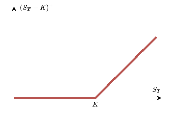
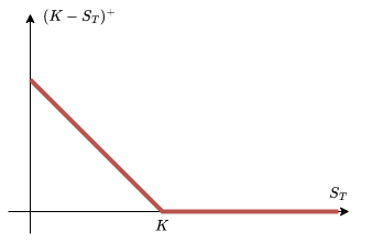
Figure 1.1: Payoff graphs for European call (left) and put (right) options with strike price \(K\).
We can also view this as \(\max (S_T - K, 0)\), which we write as \((S_T - K)^+\) (as it’s the positive part of this value).
By the same argument, the return at time T of a put option is \(\max (K - S_T, 0) = (K - S_T)^+\).
Remark. Notice that selling call options is not the same thing as buying put options! Mathematically, this is because \[ (K - S_T)^+ \not= -(S_T - K)^+\] (one side is always positive or zero, and the other is always negative or zero). In terms of the transactions, the difference arises from the fact that the choice always lies with the buyer of the option; the seller is obligated to go along with the buyer’s decision).
Exercise 1.1
Draw the graphs of the payoffs of the following combinations of options, as a function of the asset price:
- buying one call plus one put option with the same strike price \(K\) (this is known as a straddle)
- buying one call option and selling one put option with the same strike price \(K\)
- buying one call option with strike price \(K_1\), and selling another call option with strike price \(K_2\) (this is known as a bull spread; you’ll want \(K_2 > K_1\))
1.2.3 Risk
Investors in financial markets are hugely concerned with risk. Given two investments with the same expected return, investors will generally prefer the one with smaller variation. For instance, imagine you have £10,000 to invest, and you are choosing between the following strategies:
- Strategy A will return £0 with probability 0.45, or £20,000 with probability 0.55;
- Strategy B will return £10,000 with probability 0.5, or £12,000 with probability 0.5.
In both cases, the expected return is £11,000; but the variability (and hence the risk) is much higher with Strategy A. Nearly all investors would prefer Strategy B, as the potential losses are much smaller.
On the other hand, we could consider a third strategy: placing all of our money in a risk-free account, where it will sit and quietly earn interest.
- Strategy C will return £11,000 with probability 1.
Would you prefer Strategy C over Strategy B? For many investors, the low-risk (but not risk-free) option is most attractive.
In every market we study, we assume that there are opportunities for risk-free investment in the form of bonds. These bonds pay interest at a known, constant rate \(r\).
Context: nominal and effective interest
If the interest is compounded once per year, then after one year an initial deposit of \(B(0)\) will be worth \(B(1) = B(0)(1+r)\), and after \(t\) years, \(B(t) = B(0)(1+r)^t\).
If it is compounded \(n\) times per year (common choices for \(n\) include 2, 4, 12, 52, and 365) at a nominal rate \(r\), then at each of \(n\) equally-spaced intervals, the value of the investment increases by a factor \((1+r/n)\), so that \(B(1/n) = B(0)(1+r/n)\) and, more generally, \(B(m/n) = B(0) (1+r/n)^m\).
If we deposit £\(B\) in bonds at the start of the year, and interest is compounded \(n\) times at nominal rate \(r\), then after one year our investment will be worth £\(B(1+r/n)^n\). The effective interest rate is the value \(r^*\) such that \[ 1 + r^* = (1 + r/n)^n. \] If you take out a loan or a mortgage, the APR you’ll see advertised is the effective interest rate, expressed as a percentage.
Present-value analysis
Because we can always invest money into bonds for a guaranteed interest rate, a deposit of £1000 today is “worth more” than a deposit of £1000 in a year’s time. To account for this, we calculate the present value of a cash flow. To do this, we multiply each deposit by the discount factor \[\alpha =\frac1{1+r}:\] a deposit of £\(x\) at time \(t\) is worth \(x \alpha^t\) “in today’s money”.
Which of these cash flows has the highest (and the lowest) present value?
- \(x_i = 100\), \(t_i \in \{1,3,5,7,9\}\)
- \(x_i = 50\), \(t_i \in \{1, 2,3,4,5,6,7,8,9,10\}\)
- \(x_i = 200\), \(t_i \in \{1,3,5,7,9\}\) and \(x_i = -100, t_i \in \{2,4,6,8,10\}\)
- Wildcard: construct your own cash flow.
You have a bank account in which the annual interest rate is 5%, compounded monthly You plan to pay in £\(D\) every month for thirty years (360 months), and then withdraw £1000 every month for the following twenty years (months 361 - 600). What is the minimum deposit \(D\) you should be making, to ensure you have enough in your account?
Here \(r = 0.05/12 = 1/240\), so \(\alpha = 240/241\). The present value of all the deposits is \[ D + D \alpha + D \alpha^2 + \dots + D \alpha^{359} = D \sum_{i=0}^{359} \alpha^i = D \ \frac{1-\alpha^{360}}{1-\alpha}. \]
Next, the present value of all the withdrawals is \[ 1000 \alpha^{360} ( 1 + \alpha + \alpha^2 + \dots + \alpha^{239}) = 1000 \alpha^{360} \frac{1 - \alpha^{240}}{1-\alpha}. \]
These are equal when \[ D = 1000 \alpha^{360} \frac{1-\alpha^{240}}{1-\alpha} \frac{1-\alpha}{1-\alpha^{360}} = 1000 \alpha^{360} \frac{1-\alpha^{240}}{1-\alpha^{360}} \approx 182.065. \]
1.2.4 Portfolios
In general, a portfolio is a description of the shares, options, and cash we hold at any given time. The values of any of these things can be negative if we engage in short selling: borrowing units of an asset at one time, to be returned later. In this course, it is always possible to short sell anything we need to: there is always someone willing to lend it to us. This is part of an assumption of liquidity which we will discuss later.
We can describe a portfolio in one of two different ways: in terms of the amount of each asset we hold at every time \(t\), or in terms of the amount of each asset we buy or sell.
The trades defining a portfolio need not happen at deterministic (pre-determined) times. For example, we may wish to create a portfolio in which we buy shares of a stock at time 0, and then sell them as soon as the share price doubles. In that case, the time of our trade is \(\inf \ \{ t : S_t \geq 2 S_0\}\). This is a permissible trade, because we will recognise the moment when it happens; on the other hand, we can’t decide to sell “whenever the price is highest between time 0 and time \(T\)”, because we can’t know whether or not that moment has arrived. If you took Markov Chains last year, you might recognise that we’re talking about stopping times.
We say that a portfolio is self-financing if each of the trades involved produces no cash flow – that is, if the total value of what we buy is equal to the total value of what we sell. In practice, this means that we use the principle that, aside from some initial investment, the trading strategy should take care of itself.
When it is possible to assemble a portfolio that is certain to produce a profit, we say that there is an arbitrage opportunity in the market. We can think of arbitrage as arising from two different possible sources. Firstly, if an underlying asset is guaranteed to out-perform the other assets in the market (including the risk-free investment in bonds), then there is arbitrage inherent in the market. In some sense, the whole market is rigged; there’s a guaranteed win somewhere in there. Secondly, if an asset (usually a derivative asset) is mis-priced, then investors can create arbitrage by buying (or selling) the mispriced asset in large quantities, as we’ll see in the next example.
A company’s shares are floated on the stock market. The value of one share is £100 today (at \(t = 0\)), and we know that tomorrow (at \(t=1\)) the value will either increase to £200, with some unknown probability \(0 < p < 1\), or decrease to £50 with probability \(1-p\).
We are a broker trading in stocks and options, and we’re considering the following (European call) option: the holder has the right (but not the obligation) to buy one share for £150, at time \(t=1\). At time \(t=0\), what is the fair price \(C\) for this option? We have to be willing to both buy and sell options at this price, and we will assume that there’s a wealthy trader “Agent A” who will take advantage and run us out of business if we misprice the option and create an arbitrage.
One approach is to think about the value of the option at time \(t=1\): if the share price is £50, then the option is worthless and we throw it away. If the share price is £200, then by exercising the option and immediately selling the share, the holder will make a profit of £50. So the expected value of the option is \(50 p\) – to decide what \(C\) should be, we’ll need an estimate for \(p\). Let’s see what happens if we estimate that \(p=0.2\), so that \(C =\) 10.
Agent A comes along, and asks to sell us a share and buy 3 options at time \(t=0\). With this transaction, we initially hand over \[ 100 - 3 \times 10 = 70.\]
An important note here is that Agent A can sell us as many shares as he likes, through short selling. He borrows the shares from some third party at time 0, and he will have to return them at time 1. In practice, this means that for every share he sells us now, he will have to buy one back later.
At time 1, if the share price has gone down, the option is worthless. In this case, he can buy one share of the stock for £50, return it to the third party, and leave with \[ 70 - 50 = 20\] in profit.
On the other hand, if the share price has gone up, each option represents a profit of £50. In this case, Agent A will spend £450 to exercise the options; return one share to the third party; and sell the two remaining shares for £400. This time, he leaves with \[ 70 - 450 + 400 = 20 \] in profit.
In either case, Agent A has returned his borrowed share and made a £20 profit from us: there is no risk! This is an example of an arbitrage opportunity. Since Agent A has effectively limitless money, he can instead sell a million shares, buy three million options, and make £20 million profit - or even more - and ruin us.
In order to calculate the fair price for the option, we should think about Agent A’s profit in general terms. Let’s consider a portfolio consisting of \(x\) units of the stock and \(y\) units of the option; here, negative values for \(x\) and \(y\) represent short selling. The initial cost to Agent A is \[100 x + C y.\]
At time 1, this portfolio is either worth \(50x\) (if the share price goes down), or \(200 x + 50y\) (if the share price goes up). To eliminate the risk and make the two values equal to each other, we set \(y = -3x\).
Overall, this portfolio has a risk-free profit of \[ 50 x - (100 x - 3 Cx) = (3C - 50)x. \]
If this is non-zero, Agent A can ruin us! If it’s positive, he takes a hugely positive value for \(x\) (this is buying the stock and short selling the option). If it’s negative, he can take a hugely negative value for \(x\) (this corresponds to short selling the stock and buying the option, as in the first part of the example). The only way to avoid arbitrage is to set \(C= 50/3\).
A basic underlying principle of derivative pricing is:
No market should inherently contain arbitrage opportunities, and no financial derivative should be priced in a way that creates an arbitrage opportunity.
In a liquid market, arbitrage opportunities are not stable and never exist for long: investors taking advantage of the opportunity (or arbitrageurs) will influence the supply and demand within the market and push the price back towards one that does not create arbitrage.
The principle that no derivative asset should be priced in a way that leads to arbitrage opportunities allows us to conclude that larger payoffs must mean larger prices.
Proposition 1.1 Consider two self-financing portfolios, Portfolio 1 and Portfolio 2, with costs \(C_1\) and \(C_2\), and time-\(T\) payoffs \(V_1\) and \(V_2\). If \(V_1 \geq V_2\) is true whatever happens to the asset prices, then we must have \(C_1 \geq C_2\) or an arbitrage opportunity exists.
(In other words: if Portfolio 1 is a better bet than Portfolio 2, it can’t cost less.)
Proof. We use the golden principle of exploiting arbitrage opportunities: buy cheap, and (short) sell expensive.
Suppose \(C_2 > C_1\). At time \(0\), by borrowing the second portfolio, selling it, and using the money to buy the first portfolio, our position is:
- holding Portfolio 1
- short Portfolio 2
- spare cash worth \(C_2 - C_1\), which we can use to buy bonds.
Now at time \(T\), we sell Portfolio 1 for \(V_1\), pay \(V_2\) to buy Portfolio 2 and return it to the lender, and have \(V_1 - V_2 \geq 0\) left over from the transaction. In combination with the bonds which have been quietly earning interest, we are guaranteed to make a profit: this is an arbitrage opportunity.
By applying 1.1 in both directions, we obtain the Law of One Price:
Theorem 1.1 (The Law of One Price (LOOP)) If two self-financing portfolios have identical time-\(T\) payoffs, whatever happens to the asset prices, then at every time \(t \leq T\), they must have the same price or an arbitrage opportunity will exist.
An example of the Law of One Price is Put-Call Parity:
Theorem 1.2 (Put-Call Parity) Consider a European call option with cost \(C\), and a European put option with cost \(P\), on the same stock. If the initial share price is \(S_0\), interest is compounded discretely at rate \(r\), and both \(C\) and \(P\) have strike price \(K\) and expiry date \(T\), then we must have \[ P + S_0 = C + K(1+r)^{-T}, \] or else an arbitrage opportunity exists.
Proof. Consider two portfolios, \(X\) and \(Y\). In \(X\), we buy one call option and put \(K (1+r)^{-T}\) into bonds, buying \(K (1+r)^{-T}\) units, at time 0. The price at time 0 is \(C + K (1+r)^{-T}\), and at time \(T\) the portfolio will be worth \[ V_T^X = (S_T - K)^+ + K (1+r)^{-T} \times B_T = (S_T - K)^+ + K = \max(S_T, K). \]
In \(Y\), we buy one put option and one share of stock at time 0. The price at time 0 is \(P + S_0\), and at time \(T\) portfolio \(Y\) will be worth \[ V_T^Y = (K - S_T)^+ + S_T = \max(K, S_T).\]
Since both portfolios have the same payoff, they must have the same initial cost by the Law of One Price to avoid an arbitrage opportunity; so \[ C + K (1+r)^{-T} = P + S_0. \]
We say that one portfolio hedges or replicates another if they always have the same payoff. A complete market is a market in which every contingent claim can be hedged with a portfolio consisting only of bonds and shares. Using the Law of One Price, we can calculate the fair price for any derivative asset at any time by first finding a hedging portfolio using bonds and shares, and then calculating its fair price – which should be a straightforward calculation.
1.3 Discrete-time model
In this part of the course, we are interested in discrete-time models: those in which trading can take place only at specific times.
A discrete-time model with one risky asset consists of:
- A set of trading times \(0 < t_1 < t_2 < t_3 < \dots \leq T\). These do not have to be equally-spaced, but usually will be; we will almost always use \(t_j = j\) so that trades happen at times \(0,1,2,3, \dots, T\).
- An outcome space \(\Omega\). Each element of \(\Omega\) represents one possible way in which the share prices might evolve; this is how we will encode the risk or randomness in the model.
- A risk-free asset, or bonds account, whose price dynamics are deterministic and given by \[ B(t) = (1+r)^t, \qquad 0 \leq t \leq T.\]
- A risky asset, whose price dynamics are defined for each \(\omega \in \Omega\) by \[ S : \omega \mapsto \{ S_1(\omega), \dots, S_T(\omega)\}. \] The collection \(\{ S_1(\omega), \dots, S_T(\omega)\}\) represents one possible price path for the share price.
Notes:
- The outcome space \(\Omega\) should remind you of probability triples \((\Omega, \mathcal{F}, \mathbb{P})\) from Probability II. We’re going to avoid defining a probability measure on \(\Omega\) for now, but \(\mathcal{F}\) will usually be the Borel \(\sigma\)-algebra \(\mathcal{F} = 2^{\Omega}\).
- The interest rate \(r\) for the risk-free asset must be unique, to avoid arbitrage inherent in the market. If there were two different risk-free assets, with rates \(r_1 < r_2\), then a portfolio in which we short-sell one bond at the lower rate, buying one bond at the higher rate, creates a guaranteed payoff of \((1+r_2)^T - (1+r_1)^T > 0\) with no initial investment.
- We view all price paths for the shares as left-continuous functions of time: \(S_t = S_{t^-}\).
We make the following assumptions about the market:
- The market is liquid and divisible: we can buy or sell any (real) quantity of bonds and of shares at each time \(t_i\).
- We do not have to pay transaction fees, and transactions happen instantaneously at each trading time.
- There is no bid-ask spread: the prices at which we buy are the same as the prices at which we sell.
- Shares produce no dividends.
- Our actions have no impact on the pricing of any products in the market.
The second and third assumptions, together, are known as a frictionless market. They represent two of the major stumbling blocks that you will face if you set out to identify and exploit arbitrage opportunities in the real world.
In this course, we usually describe a portfolio as a sequence of holdings vectors, rather than in terms of the trades we need to make to achieve those holdings. For example, if we hold \(x\) bonds and \(y\) units of the stock at time \(t\), we have \(h_t = (x,y)\). A portfolio in which we short sell one share at time \(t=1\) and buy it back at time \(t=3\) would therefore look like: \[ h_t = \begin{cases} (0,0) & 0 \leq t < 1 \\ (0,-1) & 1 \leq t < 3 \\ (0,0) & 3 \leq t < T. \end{cases}\]
Note that this portfolio is defined at \(t=0\), but not at \(t=T\): we assume that, at time \(T\), we will exercise any contracts that are worth exercising, return anything we borrowed, and sell any remaining assets.
We can view a portfolio as a function \(t \mapsto h_t\). It’s a step function which is constant on the intervals \([0,1)\), \([1,2)\), and so on. In fact, any right-continuous piecewise step function can be seen as a portfolio, as long as the “jumps” happen only at trading times. We could also view a portfolio as a sequence of trades, rather than a sequence of holdings: to recreate the trades involved, we look for values of \(t\) for which \(h_t - h_{t^-}\) is non-zero.
The value of a portfolio at time \(t\) is given by the total value of each of the assets held; for a portfolio \(P = (h_t; t \in [0,T])\) we write \[ V_t = h_t \cdot (B_t, S_t) = x_t B_t + y_t S_t. \]
The amount of cash required to initialise a portfolio is given by \(V_0\) - note that this can be negative, for example if we’re short selling. The cash received at time \(t=T\) when we close out the portfolio is \(V_T\), which can also be negative - for example to buy back shares that were sold earlier.
If our portfolio \(X\) is “sell 100 shares of the stock at time 0”, then we can express \(X\) as a sequence of holdings by \[ X = ( h_t^X, t \in [0,T]) \qquad \qquad \mbox{where} \qquad h_t^X = (0, -100 ) \ \forall t \in [0,T].\] The value of \(X\) is always \(V_t = -100 S_t\).
If our portfolio \(Y\) is “buy 100 shares at time 0, and sell them as soon as the share price doubles”, then the holdings are given by \[ h_t^Y = \begin{cases} 100 & \sup_{s \in [0,t]} (S_s) < 2 S_0 \\ 0 & \sup_{s \in [0,t]} (S_s) \geq 2 S_0 \end{cases}.\] We can write this as \(h_t^Y = 100 \ \ind \ \{ \sup_{s \in [0,t]} (S_s) < 2 S_0 \}\). Similarly, the value of the portfolio is given by \(V_t = 100 S_t \ \ind \ \{ \sup_{s \in [0,t]} (S_s) < 2 S_0 \}\).
Question: what are the trades, holdings, and value of the portfolio \(X+Y\)?
The cash flow associated with a portfolio describes how its value changes as each trade occurs: if the portfolio has trades at times \(t_1, \dots, t_k\) and associated changes in value \(c_1, \dots, c_k\), then the cash flow is \(\{ (c_i, t_i)\}\).
We say that a portfolio is self-financing if the cash flow associated with it is trivial; in other words, if \(V_t = V_{t^-}\) for every \(t \in (0,T]\). Since \(B_t\) and \(S_t\) are left-continuous, we have \[ \begin{aligned} V_t - V_{t^-} &= x_t B_t + y_t S_t - (x_{t^-} B_{t^-} + y_{t^-}S_{t^-}) \\ & = (x_t - x_{t^-}) B_t + (y_t - y_{t^-}) S_t. \end{aligned} \]
The self-financing condition means that this value should always be 0.
Note that we can find a self-financing version of any portfolio by buying or selling bonds in the appropriate quantities to create a trivial cash flow. Although bonds are not the same as cash in practice, they play the same role in our mathematical model.
The present value profit of a self-financing portfolio \(P\) with value \(V_t, t \in [0,T]\) is given by \(\alpha^T V_T - V_0\). Remember that \(\alpha\) is the discount factor per time period, so that \(\alpha = (1+r)^{-1}\) if interest is compounded discretely at rate \(r\) per time period, or \(\alpha = e^{-r}\) if interest is compounded continuously.
We say that a portfolio \(P\) is an arbitrage portfolio if \(\alpha^T V_T - V_0 \geq 0\), whatever happens to \(S_t\), and it is possible that \(\alpha^T V_T - V_0 > 0\).
Alternatively, we can define an arbitrage portfolio as one which satisfies: (i) \(P\) is self-financing; (ii) \(V_0 = 0\); and (iii) \(V_T \geq 0\) whatever happens to the share prices and it is possible that \(V_T > 0\).
Lemma 1.1 These two definitions of an arbitrage portfolio are equivalent, in the sense that a market either allows both to exist, or neither.
The proof of this Lemma is Exercise 1.10 on the problem sheet.