Chapter 3 The multi-period binomial model: Part 1

3.1 Introduction

In this chapter, we extend the one-period binomial model to allow for more trading times. Our model becomes:

A set of trading times, \(\{0,1,2,\dots, T\}\).
An outcome space, \(\Omega = \{0, 1\}^T\).
A bond, with price dynamics: \[ B(0) = 1, \qquad \qquad B(t) = (1+r)^t.\]
A share, whose price dynamics are: \[ S_0(\omega) = s, \quad \text{for all } \omega \in \Omega, \] and for each \(t = 1, 2, \dots, T\), \[ S_t(\omega) = Z_t(\omega) S_{t-1}(\omega),\] where \(Z_1, Z_2, \dots, Z_T\) are random variables defined on \(\Omega\), with \[ Z_t(\omega) = \begin{cases} u & \text{if } \omega_t = 1, \\ d & \text{if } \omega_t = 0. \end{cases} \]

Notes:

In this model, \(\Omega\) is the set of all sequences of length \(T\), in which each element is a 0 or a 1. The sequence 00…0 corresponds to the share price moving “down” \(T\) times, while the sequence 11…1 corresponds to the share price moving “up” \(T\) times. When we discuss an element \(\omega \in \Omega\), we will sometimes write \(\omega = \omega_1 \omega_2 \dots \omega_T\).
The Borel \(\sigma\)-algebra on \(\Omega\) is \(\mathcal{F}_T = 2^{\Omega}\) and consists of all possible subsets of the \(2^T\) elements of \(\Omega\). For instance \(\{ \omega \in \Omega: \omega_1 = 0\} \in \mathcal{F}_T\). More on this later.
As before, the price dynamics of the risk-free asset evolve deterministically via the risk-free interest rate.
We assume that \(S_0>0\) is fixed, and that if we know the share price is \(S_t\) at time \(t\), there are two possible values for the share price at time \(t+1\): \(S_t \times u\) and \(S_t \times d\). Although we will sometimes work with models in which \(u\) and \(d\) take the same values for all \(t\) and \(s\), this is not necessarily the case, as you will see in Example 3.1.

Consider a two-period model with the possible share prices \(S_t, t=0,1,2,\) given by the tree:

A tree diagram, with prices 120 and 60 at time 1, and 180, 80, 72, and 36 at time 2.

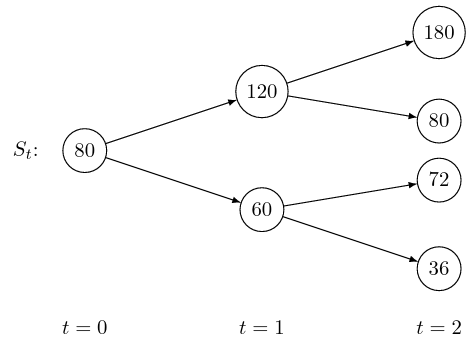
At \(t=0\), we have \[ u=\frac{120}{80}=\frac{3}{2} \qquad \mbox{and} \qquad d=\frac{60}{80}=\frac{3}{4}. \]
At \(t=1\), when \(S_1=120\), we have \[u=\frac{180}{120}=\frac{3}{2} \qquad \mbox{and} \qquad d=\frac{80}{120}=\frac{2}{3}.\]
At \(t=1\), when \(S_1 = 60\), we have \[u=\frac{72}{60}=\frac{6}{5} \qquad \mbox{and} \qquad d=\frac{36}{60}=\frac{3}{5}. \]

As in the one-period version of the model, the values of \(p_u\) and \(p_d\) do not matter to us, as long as \(0 < p_u, p_d < 1\). For this reason, we do not ask whether \(p_u\) always takes the same value regardless of \(t\) and \(s\); both possibilities are entirely reasonable.

The multi-period binomial model is free from inherent arbitrage if and only if there is no inherent arbitrage to be found by considering any of its constituent parts. In other words, it is free from inherent arbitrage as long as \[ d < 1+r < u\] holds everywhere in the model.

A portfolio on a multi-period market is now more complicated to describe, since we need to specify the amounts we hold of each asset at each time \(t\), and this is allowed to depend on how the share price changes over time. However, we can still price contingent claims in this model, by using the risk-neutral valuation formula to find the no-arbitrage price at each node of the tree.

3.2 Portfolios and the self-financing condition

In this market, a portfolio is a sequence of pairs of random variables \(h_t = (x_t, y_t)\), \(t =1, \dots, T\). Each pair is interpreted as follows:

\(x_t\) is the number of units of the risk-free asset in your portfolio at time \(t-1\) and kept until time \(t\).
\(y_t\) is the number of units of the risky asset in your portfolio at time \(t-1\) and kept until time \(t\).

The amounts \(x_t\) and \(y_t\) can depend on the present and past history \(S_0, S_1, \dots, S_{t-1}\) of the stock prices; it is reasonable to assume that we can find functions \(f_x\) and \(f_y\) such that \[ x_t = f_x(S_0, \dots, S_{t-1}) \qquad y_t = f_y(S_0, \dots, S_{t-1}). \]

Consider a market with \(T=2\), in which the time-0 share price is 10, at time 1 the share price will either be 15 or 8, and at time 2 the share price will be 18, 12, or 6. For this example, we use \(r = 0\).

Our portfolio is “buy 20 shares at time 0; at time 1, sell half (and buy bonds) if the price goes up, or sell all of them if the price goes down”.

In either case, we short sell \(20\times10=200\) bonds to buy the initial shares; at time 1, we use the cash from our sale to buy either \(10\times 15=150\) or \(20\times 8=160\) bonds.

To express this portfolio as a sequence of vectors, we write: \[ \begin{aligned} \text{at time }0, \qquad &(x_1,y_1) = (-200,20) \\ \text{at time } 1, \qquad &(x_2,y_2) = \begin{cases} (-50,10) \qquad \text{ if }\omega_1 = 1 \\ (-40,0) \qquad \,\,\, \text{ if }\omega_1 = 0. \end{cases} \end{aligned}\]

The value of a portfolio at time \(t = 0, \dots, T\) is given by \[ V_t = x_{t+1} B_t + y_{t+1} S_t, \] with the convention that \(x_{T+1} = x_T\) and \(y_{T+1} = y_T\). In other words, this is the value of the portfolio after the trade at time \(t\), and before the next price change.

In the market in the previous example, if \(\omega_1 = 1\) (so the share price increases to 15 at time 1), then the value of the portfolio at time 1 is \[ V_1^h = x_2 B_1 + y_2 S_1 = -50 + 10 \times 15 = 100.\]

Between times \(t-1\) and \(t\), the values of the bond and the stock change from \(B_{t-1}\) and \(S_{t-1}\) to \(B_t\) and \(S_t\), so that the portfolio is now worth \(x_t B_t + y_t S_t\); we adjust our holdings according to the price changes, so that we now hold \((x_{t+1}, y_{t+1})\). This adjustment is self-financing if \[\begin{equation} x_tB_t+y_tS_t=x_{t+1}B_t+y_{t+1}S_t. \tag{3.1} \end{equation}\] If (3.1) holds for all \(t=1,\dots,T\), we say the portfolio is self-financing. This condition basically means that you cannot take out money from the portfolio or put in money to the portfolio: it should finance itself.

Remark. Using the expression for the value \(V_t\) of the portfolio at time \(t\), the self-financing constraint (3.1) can be rewritten as the condition \[\begin{equation} V_t-V_{t-1}=x_t(B_t-B_{t-1})+y_t(S_t-S_{t-1}). \tag{3.2} \end{equation}\] The financial meaning of this is that the change in the value \(V_t-V_{t-1}\) of a self-financing trading strategy is due only to the gains/losses \[ x_t(B_t-B_{t-1})+y_t(S_t-S_{t-1}) \] due to price changes of the assets. Summing both sides of (3.2) over \(t\) we obtain \[ V_T-V_0=\sum_{t=1}^T (V_t-V_{t-1})=\sum_{t=1}^T x_t[B_t-B_{t-1}]+\sum_{t=1}^T y_t[S_t-S_{t-1}]. \] You will see this form when we start to define stochastic integration and self-financing conditions in continuous time.

3.3 The martingale measure

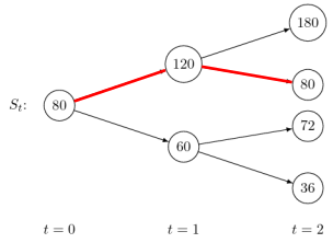
To construct the martingale measure in this model, we take the product measure based on the martingale measure found in Chapter 2. To find \(\mathbb{Q}(\omega)\), we trace out the path represented by \(\omega\) in the pricing tree. We calculate the one-step martingale measures at each node, and multiply them together.

In the market from Example 3.1, the choice \(\omega = 10\) represents the share price increasing in the first instance, and decreasing in the second:

At \(t=0\), we have \[ q_u = \frac{1 - \frac{3}{4}}{\frac{3}{2} - \frac{3}{4}} = \frac{1}{3} \qquad \mbox{and} \qquad q_d = \frac{\frac{3}{2} - 1}{\frac{3}{2} - \frac{3}{4} } = \frac{2}{3}.\]

At \(t=1\) and \(S_1 =120\), we have \[ q_u = \frac{1 - \frac{2}{3}}{\frac{3}{2} - \frac{2}{3}} = \frac{2}{5} \qquad \mbox{and} \qquad q_d = \frac{\frac{3}{2} - 1}{\frac{3}{2} - \frac{2}{3}} = \frac{3}{5}. \]

So \[ \mathbb{Q}(\omega = 10) = \frac{1}{3} \times \frac{3}{5} =\frac{1}{5}.\]

Next, for \(A \in \mathcal{F}\),we define \(\mathbb{Q}(A)\) using the elements \(\omega \in A\): \[ \mathbb{Q}(A) = \sum_{\omega \in A} \mathbb{Q}(\omega).\]

Exercise 3.1

“Prove” (convince yourself) that constructing the product measure in this way makes sense: all the probabilities are non-negative and add up to 1, and we have \(\mathbb{Q}\left(\omega_1=1\right) = q_u\) and \(\mathbb{Q}\left(\omega_1=0 \right) = q_d\) as expected.

Suggestion: in the model with \(T=2\), calculate \(\mathbb{Q}(11)\) and \(\mathbb{Q}(10)\) and check that they add up to \(q_u\). Do the same calculation for \(T=3\), and then think about the general case.

3.4 Pricing European contingent claims

3.4.1 Pricing contingent claims via the risk-neutral valuation formula

We work from \(t=T-1\) to \(t=0\), using backwards induction.

We denote the price of a contingent claim \(X= \Phi(S_T)\), evaluated at time \(t\), by \(\Pi(X,t)\). We will also sometimes use the notation \(\Pi_t(\Phi)\).

Let’s focus on a single node of the tree. Suppose that the share price at time \(t\) is \(S_t = s\), and the two possible values for \(S_{t+1}\) are \(su\) and \(sd\). We also suppose that we know the two possible values for the fair price for the contingent claim at time \(t+1\). We denote these \(\Pi^u_{t+1}\) and \(\Pi^d_{t+1}\) .

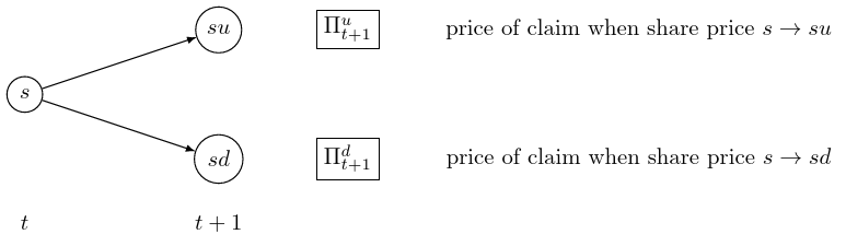
Using the same approach as in Chapter 2, we can find the martingale probabilities: \[ q_u = \frac{1+r-d}{u-d} \qquad q_d = \frac{u-(1+r)}{u-d}, \] and then the price \(\Pi_t\) at time \(t\) is given by \[ \Pi_t = \frac{1}{1+r} \left( q_u \Pi^u_{t+1} + q_d \Pi^d_{t+1} \right). \]

Working through all the nodes in this way, we can eventually find \(\Pi_0\) as a linear combination of \(\Pi^u_1\) and \(\Pi^d_1\).

For the market in Example ??, with \(r=0\), let’s calculate the fair price of a European call option with expiry date \(T=2\) and strike price \(K=70\).

First, we find the martingale measure:

at \(t=0\), we have \[ q_u = \frac{1 - \frac{3}{4}}{\frac{3}{2} - \frac{3}{4}} = \frac{1}{3} \qquad \mbox{and} \qquad q_d = \frac{\frac{3}{2} - 1}{\frac{3}{2} - \frac{3}{4} } = \frac{2}{3}.\]
at \(t=1\) and \(S_1 =120\), we have \[ q_u = \frac{1 - \frac{2}{3}}{\frac{3}{2} - \frac{2}{3}} = \frac{2}{5} \qquad \mbox{and} \qquad q_d = \frac{\frac{3}{2} - 1}{\frac{3}{2} - \frac{2}{3}} = \frac{3}{5}. \]
at \(t=1\) and \(S_1 = 60\), we have \[ q_u = \frac{1 - \frac{3}{5}}{\frac{6}{5} - \frac{3}{5}} = \frac{2}{3} \qquad \mbox{and} \qquad q_d = \frac{\frac{6}{5} - 1}{\frac{6}{5} - \frac{3}{5}} = \frac{1}{3}. \]

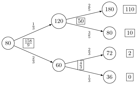
Now, we work backwards to find the price of the option at each node. When \(t=2\), we know that \(\Pi_2 = (S_2 - 70)^+\), so that the option is worth \(110, 10, 2,\) or \(0\), when \(S_2\) equals \(180, 80, 72,\) and \(36\), respectively.

Now when \(t=1\) and \(S_1 = 120\), we have \[ \begin{aligned} \Pi_1 &= \frac{1}{1+r} \left( q_u \Pi^u_2 + q_d \Pi^d_2 \right) \\ & = \frac{1}{1+0} \left( \frac{2}{5} \times 110 + \frac{3}{5} \times 10 \right) \\ & = 50. \end{aligned}\]

When \(t=1\) and \(S_1 = 60\), we have \[ \begin{aligned} \Pi_1 &= \frac{1}{1+r} \left( q_u \Pi^u_2 + q_d \Pi^d_2 \right) \\ & = \frac{1}{1+0} \left( \frac{2}{3} \times 2 + \frac{1}{3} \times 0 \right) \\ & = \frac{4}{3}. \end{aligned}\]

Finally, we \(t=0\), we have \[ \begin{aligned} \Pi_0 &= \frac{1}{1+r} \left( q_u \Pi^u_1 + q_d \Pi^d_1 \right) \\ & = \frac{1}{1+0} \left( \frac{1}{3} \times 50 + \frac{2}{3} \times \frac{4}{3} \right) \\ & = \frac{158}{9}; \end{aligned}\] so the no-arbitrage price of the call option is \(\frac{158}{9}\).

These calculations are often recorded in a single tree: we write the share prices inside the nodes, the martingal probabilities along the arrows, and the prices of the claim next to each node in rectangles.

Once we have calculated the martingale probabilities at each node, the martingale measure for \(S_T\) is the product measure \(\mathbb{Q}\), which we obtain by multiplying the probabilities along each arrow. For instance, in Example ??, \(\mathbb{Q}(S_T = 180) = \frac13 \times \frac25 = \frac{2}{15}\). Under this measure, we have \[ S_0 = \frac{1}{(1+r)^T} \mathbb{E}_{\mathbb{Q}} [S_T], \] and we can view the initial price \(\Pi_0(\Phi)\) as the present value of the expectation of \(\Phi(S_T)\): \[ \Pi_0(\Phi) = \frac{1}{(1+r)^T} \mathbb{E}_{\mathbb{Q}} [\Phi(S_T)]. \]

Warning: of course you already know this, but \(\mathbb{E}_{\mathbb{Q}} [\Phi(S_T)]\) is not the same thing as \(\Phi\big(\mathbb{E}_{\mathbb{Q}} [S_T]\big)\).

Consider the market as described in Examples ?? and ??. Using the martingale probabilities on each arrow, we can calculate the martingale measure \(\mathbb{Q}\) for \(S_2\) (here \(T=2\)). For example, the stock price \(S_2\) equals 180 exactly when the price \(S_t\) follows the path \(80 \to 120 \to 180\) through the tree, so \(\mathbb{Q}(S_2 = 180) = \frac13\times\frac25 = \frac2{15}\). There are a total of 4 possible values that \(S_2\) can take: 180, 80, 72 or 36, and these have probabilities \(\frac2{15}, \frac15, \frac49\) and \(\frac29\).

The expectation of \(S_2\) with respect to this measure is \[\mathbb{E}_{\mathbb{Q}}[S_2] = \frac2{15}\times 180 + \frac15 \times 80 +\frac49 \times 72 +\frac29 \times 36 = 80.\]
As expected this equals \(S_0\), since in this example \(r=0\).

Now, to find the price \(\Pi_0\) at time 0 of the call option with strike price 70 and expiry date \(T=2\), we calculate the present value of the expectation under \(\mathbb{Q}\) of the value at time \(T\) of the call option, \((S_2-70)^+\). We find that \[\mathbb{E}_{\mathbb{Q}}[(S_2-70)^+] = \frac2{15}\times 110 + \frac15 \times 10 +\frac49 \times 2 +\frac29 \times 0 = \frac{158}9, \] which agrees with our previous calculation.

3.4.2 Pricing contingent claims by hedging

For now, we will focus on European claims – that is, claims whose contract functions are of the form \(X = \Phi(S_T)\). In Chapter 5, we will extend our theory to include claims in which the payoff can depend on the past history of the stock price.

Theorem 3.1 For a contingent claim \(X\), suppose that there exists a self-financing trading strategy \(h_t = (x_t, y_t)\), \(t= 1, 2, \dots, T+1\) whose value process \(V_t^h\), \(t = 0, \dots, T\) satisfies \[ \mathbb{P} (V_T^h = X ) = 1. \] Then for each \(t = 0, 1, \dots, T\), we must have \[ \Pi_t(\Phi) = V_t^h, \] or else the market will contain arbitrage.

Proof. We first suppose that \(V_t^h < \Pi_t(\Phi)\) holds for some \(t\). Then, at this time, we can (short) sell the contingent claim and use the money to buy the portfolio, using the remaining \(\Pi_t(\Phi) - V_t^h\) to buy bonds.

Now at time \(T\), the value of our short-sold contingent claim is exactly covered by our portfolio, and we have a risk-free profit of \([\Pi_t(\Phi) - V_t] (1+r)^{T-t}\).

Similarly, if \(V_t^h > \Pi_t(\Phi)\), we can buy the contingent claim and sell the portfolio, and obtain a risk-free profit of \([V_t - \Pi_t(\Phi) ] (1+r)^{T-t}\).

We can now construct the hedging portfolio for any claim, by backwards induction from \(t=T\). We know the price of the claim at all nodes at time \(T\); to move backwards in time by one step, we need to find \(x_t\) and \(y_t\) such that \[ x_{t-1} B_{t-1} + y_{t-1} S_{t-1} = V_{t-1} = x_{t} B_{t-1} + y_{t} S_{t-1} \] holds, whichever node we reach at time \(t\). The two possiblities give us two equations in two unknowns:

\[\begin{align*} x_t(1+r)B_{t-1} + y_t S_{t-1}u &= \Pi^u_t,\\ x_t(1+r)B_{t-1} + y_t S_{t-1}d &= \Pi^d_t, \end{align*}\] which we can solve to get \[\begin{equation} x_t = \frac{1}{(1+r)B_{t-1}}\frac{u\Pi^d_t - d\Pi^u_t}{u-d}, \quad y_t = \frac{\Pi^u_t-\Pi^d_t}{S_{t-1}u-S_{t-1}d}. \tag{3.3} \end{equation}\] We can check that \[\begin{equation} \begin{split} \Pi_{t-1} = V_{t-1} = x_tB_{t-1} + y_tS_{t-1} &= \frac{1}{1+r}\frac{u\Pi^d_t - d\Pi^u_t}{u-d} + \frac{\Pi^u_t-\Pi^d_t}{u-d}\\ &= \frac{1}{1+r} [ q_u \Pi^u_t + q_d \Pi^d_t], \end{split} \tag{3.4} \end{equation}\] recalling that the martingale probabilities are \(q_u = \displaystyle\frac{1+r-d}{u-d}, q_d = \frac{u-(1+r)}{u-d}\).

We can repeat these calculations at every node at time \(t-1\) (remembering that the values of \(u\) and \(d\) might be different at different nodes), to find the price \(V_{t-1} = \Pi_{t-1}(\Phi)\) and the portfolio \((x_t,y_t)\) at every node at time \(t-1\).

So, starting at time \(T\), we use Equations (3.3) to find \((x_T,y_T)\) at every node at time \(T-1\) so that the value of the portfolio matches the prices \(\Pi_T(\Phi)\) at time \(T\). We calculate the value of this portfolio \(V_{T-1}\), which then must be equal to the price of the claim \(\Pi_{T-1}(\Phi)\) at time \(T-1\). Then, using our inductive step for \(t=T-1,T-2,\dots,1\), we can find the price of the claim and the portfolio at every node of the tree.

Remark. Just as in the one-period case, we can use the martingale measure to calculate the fair price for the claim without finding the hedging portfolio, through Equation (3.4).

Let’s calculate the hedging portfolio for the call option from Example ??. We will use the fair prices of the call option at each time, that we calculated earlier.

We start at time \(t=1\), with the case \(S_1 = 120\). We need to find \((x_2, y_2)\) such that the value of the portfolio matches the fair price of the option (either 110 or 10) at time 2. Since \(r=0\), we have \(B_t = 1\) for all \(t\) and Equations (3.3) become \[ x_2 = \frac{\frac32\times10 - \frac23\times 110}{\frac32-\frac23} = -70,\quad y_2 = \frac{110 - 10}{180-80} = 1, \] and we have \[ V_1 = x_2 + 120y_2 = -70 + 120\times 1 = 50,\] which matches the fair price for the claim we found earlier.

If instead, \(S_1 = 60\), then our \((x_2, y_2)\) will need to give values of either 2 or 0 at time 2. Now Equations (3.3) give \[ x_2 = \frac{\frac65\times0 - \frac35\times 2}{\frac65-\frac35} = -2,\quad y_2 = \frac{2 - 0}{72-36} = \frac{1}{18}, \] and \[V_1 = x_2 + 60y_2 = -2 + 60\times\frac1{18} = \frac43, \] so again we have matched the price of the claim.

Now at time \(t=0\), we need to find \((x_1, y_1)\) giving values of either 50, if the share price goes up, or 4/3, if the share price goes down. We find \[ x_1 = \frac{\frac32\times\frac43 - \frac34\times 50}{\frac32-\frac34} = -\frac{142}3,\quad y_1 = \frac{50 - \frac43}{120-60} = \frac{73}{90}, \] and we have \[V_0 = x_1 + 80y_1 = -\frac{142}3 + 80\times\frac{73}{90} = \frac{158}9. \]

Our hedging portfolio is: \[ \begin{aligned} \text{at time }0, \qquad &(x_1,y_1) = (-\frac{142}3,\frac{73}{90}) \\ \text{at time } 1, \qquad &(x_2,y_2) = \begin{cases} (-70,1) \qquad \text{ if }\omega_1 = 1 \\ (-2,\frac{1}{18}) \qquad \text{ if }\omega_1 = 0. \end{cases} \end{aligned}\]

We can check the self-financing condition: if the share price goes up, then \[ x_1 + 120 y_1 = -\frac{142}{3} + 120 \times \frac{73}{90} = 50 \] and \[x_2 + 120 y_2 = -70 + 120 \times 1 = 50. \]

Similarly, if the share price goes down, then \[ x_1 + 60 y_1 = -\frac{142}{3} + 60 \times \frac{73}{90} = \frac{4}{3} ,\] and \[ x_2 + 60 y_2 = -2 + 60 \times \frac{1}{18} = \frac{4}{3}. \]

Our portfolio, consisting of \((x_1, y_1)\) and two possible outcomes for \((x_2, y_2)\) is self-financing, and replicates the returns of the random variable \((S_T - 70)^+\), whatever happens to the share prices.

3.5 Recombinant trees

In this section, we consider the special case where \(u\) and \(d\) have the same values at every node. This means that, for example, if the stock moves up and then down, it will have the same value as if it moved down and then up. We can represent the model using a diagram which has \(t+1\) nodes at each time \(t\), rather than \(2^t\), as in Figure 3.1. In this situation, we say that the diagram is recombinant (and in fact, it is no longer a tree).

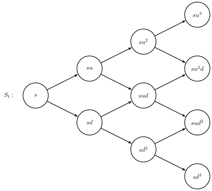
Figure 3.1: A recombinant ‘tree’.

Now, the possible values of the share price at time \(t\) are \[ S_t \in \{ s u^k d^{t-k}, \quad k=0,1,\dots,t \}, \] where \(k\) denotes the total number of up-moves that have occurred (up to time \(t\)). This means that we can specify each node in the tree by a pair \((t,k)\) with \(k=0,1,\dots,t\).

The contingent claim \(\Phi(S_T)\) can be replicated using a self-financing portfolio. If \(V_t(k)\) denotes the value of the portfolio at node \((t,k)\), then \(V_t(k)\) can be computed recursively by \[\begin{equation} \begin{split} V_T(k) &= \Phi(su^kd^{T-k}), \\ V_t(k) &= \frac{1}{1+r}[q_u V_{t+1}(k+1) + q_d V_{t+1}(k)]. \end{split} \tag{3.5} \end{equation}\] where just as before \(q_u\) and \(q_d\) are the martingale probabilities at a node, given by \[ q_u = \frac{1+r-d}{u-d}, \quad q_d = \frac{u-(1+r)}{u-d}. \] (In fact, these are the martingal probabilities at every node, since \(u\) and \(d\) are fixed.)

We can also calculate the hedging portfolio: writing \(x_t(k)\) and \(y_t(k)\) for the amounts held at node \((t-1,k)\), we have \[ x_t(k) = \frac{1}{(1+r)^t}\frac{uV_t(k) - dV_t(k+1)}{u-d}, \quad y_t(k) = \frac{V_t(k+1) - V_t(k)}{su^kd^{t-1-k}(u-d)}. \]

The recursive equations (3.5) are sometimes referred to as the binomial algorithm. We can use this algorithm to work out the fair price of a contingent claim at time 0, by starting with the nodes at time \(t=T\) and working backwards to \(t=0\). This gives us the following result.

Theorem 3.2 The arbitrage-free price at \(t=0\) of a contingent claim \(\Phi(S_T)\) is given by \[ \Pi_0(\Phi) = \frac{1}{(1+r)^T}\mathbb{E}_{\mathbb{Q}}(\Phi(S_T)), \] where \(\Q\) is the martingale measure for \(S_T\). More explicitly, we can write \[ \Pi_0(\Phi) = \frac{1}{(1+r)^T}\sum_{k=0}^T\binom{T}{k}q_u^kq_d^{T-k}\Phi(su^kd^{T-k}). \]

Proof. It is straightforward to check that the two expressions for \(\Pi_0(\Phi)\) are equivalent, by calculating \(\mathbb{Q}(S_T = s u^k d^{T-k})\). This is the probability that there are exactly \(k\) up steps, and \(T-k\) down steps, among the \(T\) total steps, so is \(\binom{T}{k}q_u^kq_d^{T-k}\). In other words, under the measure \(\Q\), the price \(S_T\) equals \(S_0u^Yd^{T-Y}\), where \(Y \sim \Bin(T,q_u)\), and therefore \[ \mathbb{E}_{\mathbb{Q}}[\Phi(S_T)] = \mathbb{E}[\Phi(S_0 u^Y d^{T-Y}) ] = \sum_{k=0}^T\Phi(S_0 u^kd^{T-k})\P[Y = k]. \]

It is also easy to see that the explicit expression for \(\Pi_0(\Phi)\) follows by applying the equations (3.5). Indeed, it is possible to show by induction on \(t\), that the value \(V_{T-t}(i)\) of the portfolio at a node \((T-t,i)\), for \(T-t \in [0,T]\) and \(i=0,\dots,T-t\), satisfies \[ V_{T-t}(i) = \frac{1}{(1+r)^t}\sum_{k=0}^t\binom{t}{k}q_u^kq_d^{t-k}\Phi(su^{i+k}d^{T-i-k}), \] and then by the Law of One Price, we have that \(\Pi_0(\Phi) = V_0(0)\), which gives the required expression.

Exercise: work out the above proof by induction. Hint: in the inductive step use the identity \(\binom{t}{k-1}+\binom{t}{k}=\binom{t+1}{k}\).

3.6 The Cox–Ross–Rubinstein formula

We use the pricing formula we found in the previous section to give a formula for the price of a European call option, known as the Cox–Ross–Rubinstein formula.

As usual, let \(K\) be the strike price of the call option, and \(T\) the expiry date. The Cox–Ross–Rubinstein formula for the price of such a call option assumes that the underlying stock can be modelled by the recombinant tree model we studied in the previous section, for appropriate choices of \(u, d\) and \(r\). As it stands, we haven’t yet considered how suitable the binomial model is as a model of stock price fluctuations. We’ll look at this question in Chapter 5, but for now we suppose that we have some appropriately chosen values for \(u, d\) and \(r\), and we price the option in terms of these parameters.

We can use the formula from Theorem 3.2 to price the call option, by setting \(\Phi(S_T) = (S_T - K)^+\). In fact, we give a more general form, for the price at time \(T-t \in [0,T]\).

Theorem 3.3 (Cox-Ross-Rubinstein formula) The price at time \(T-t\) of a European call option with strike price \(K\) and expiry date \(T\) is given by \[\begin{equation} \Pi_{T-t} = S_{T-t} \sum_{k=k^\star}^t \binom{t}{k} m_u^k m_d^{t-k} - \frac{K}{(1+r)^t} \sum_{k=k^\star}^t \binom{t}{k} q_u^k q_d^{t-k}, \tag{3.6} \end{equation}\] where \(q_u,q_d\) are the risk-neutral probabilities, \(\displaystyle m_u = \frac{q_u u}{1+r}, m_d = \frac{q_d d}{1+r}\) and \(k^\star\) is the smallest integer \(k\) that satisfies \[\begin{equation} k \log\left(\frac{u}{d}\right) > \log\left(\frac{K}{S_{T-t}d^t}\right). \tag{3.7} \end{equation}\]

Proof. The price \(\Pi_{T-t}(\Phi)\) at time \(T-t\) of the claim \(\Phi(S_T)\) is a function of the share price \(S_{T-t}\) given by \[ \frac{1}{(1+r)^t} \sum_{k=0}^t \binom{t}{k} q_u^k q_d^{t-k} \Phi(S_{T-t}u^kd^{t-k}). \] Since \(\Phi(x) = (x - K)^+\), the terms appearing in this sum will be zero unless \(S_{T-t}u^kd^{t-k} > K\). We can rewrite this condition as \((u/d)^k > K/(S_{T-t}d^t)\), and since \(u/d > 1\), there is a smallest integer \(k^\star\) given by (3.7), such that if \(k \geq k^\star\) then the condition is satisfied. (Note that if \(k^\star > t\) then the sum becomes zero, and \(\Pi_{T-t} = 0\).)

In other words, we can write the price of a European call option as \[ \Pi_{T-t} = \frac{1}{(1+r)^t}\sum_{k=k^\star}^t \binom{t}{k}q_u^kq_d^{t-k}(S_{T-t}u^kd^{t-k} - K) \] and multiplying out the bracket and using the expressions for \(m_u\) and \(m_d\) yields the formula (3.6).

Consider a 3-period model with \(u=1.2\), \(d=0.8\) and \(r=0.1\). Suppose the share price at time 0 is \(S_0 = 100\). We calculate the CRR price at time 0 of a European call option with strike price 70 and expiry date \(T=3\).

First, we calculate the martingale probabilities: \[ q_u = \frac{1.1 - 0.8}{1.2-0.8} = \frac34, \quad q_d = \frac{1.2 - 1.1}{1.2-0.8} = \frac14. \]

Then, we calculate \(m_u\) and \(m_d\): \[ m_u = \frac34\times\frac{1.2}{1.1} = \frac9{11}, \quad m_d = \frac14\times\frac{0.8}{1.1} = \frac2{11}. \]

To find the correct value of \(k^\star\), we look at the possible values for the share price at time \(T\). We see that \(S_3\) can be one of 51.2, 76.8, 115.2 or 172.8, and so the call option only has positive value at time \(T\) if at least one up-move occurs, so \(k^\star = 1\).

(Alternatively, we can calculate \(\log(K/S_0d^3) / \log(u/d) = \log(70/51.2) / \log(3/2) \approx 0.771\), and find that the smallest integer greater than this is \(k^\star = 1\).)

Then the CRR price is given by \[ \begin{aligned} V_0 &= S_0 \sum_{k=1}^3 {\textstyle\binom{3}{k}} m_u^k m_d^{3-k} - \frac{K}{(1+r)^3} \sum_{k=1}^3 {\textstyle\binom{3}{k}} q_u^k q_d^{3-k} \\ &= 100\times \frac{1323}{1331} - \frac{70}{1.331} \times \frac{63}{64} = \frac{253575}{5324} \approx 47.63. \end{aligned} \]

Remark. Note that \(m_u, m_d > 0\) and \(m_u+m_d = \displaystyle\frac{q_uu}{1+r} + \frac{q_dd}{1+r} = 1\), so that \(m_u\) and \(m_d\) can also be interpreted as probabilities. Hence we can write (3.6) as \[ \Pi_{T-t} = S_{T-t} \P[ X_t \geq k^\star ] - \frac{K}{(1+r)^t} \P[ Y_t \geq k^\star ], \] where \(X_t\) and \(Y_t\) are Binomial random variables: \(X_t \sim \Bin(t,m_u), Y_t \sim \Bin(t,q_u)\).