Practical 1-2: Sampling and Simulation
In this practical, we introduce the ideas of statistical simulation as a mechanism to investigate the behaviour of sampling distributions in a case study problem of jury selection. We’ll expand our R techniques to see how to write custom functions, to sample and generate random numbers, and how to repeat straightforward calculations an arbitrary number of times.
- Download the R Script - Right click, and Save As
- You will need the following skills from previous practicals:
- Basic R skills with arithmetic, functions, etc
- Manipulating and creating vectors:
c,seq, - Calculating data summaries:
mean,sd,var,min,max - Plotting a histogram with
hist
- New R techniques:
- Sampling from a vector using
sample - Generating random numbers from a binomial distribution using
rbinom - Creating new functions with
function - Using
replicateto repeatedly call a function with no arguments - Adding straight lines to plots with
abline
- Sampling from a vector using
1 Jury selection: Swain vs. Alabama (1965)
The context of our problem today is concerns the selection of a jury in a trial in 1965 Alabama, USA. In the early 1960s, in Talladega County in Alabama, a Black man called Robert Swain was convicted and was sentenced to death. At the time, only men aged 21 or older were allowed to serve on juries in Talladega County, where 26% of the eligible jurors were Black. Of the 100 jurors available in the jury panel, only 8 were Black and no Black man was selected for the jury of the actual trial itself.
Robert Swain appealed his sentence, citing among other factors the fact the jury at his trial was all White. Moreover, he pointed out that all Talladega County jury panels for the past 10 years had contained only a small percent of Black panelists. Robert Swain was represented in the U.S. Supreme Court by Constance Baker Motley, the first African-American woman to argue a case in that Court. She argued 10 cases in the Supreme Court and lost only one – Robert Swain’s. The U.S. Supreme Court concluded, “the overall percentage disparity has been small” and that there was insufficient evidence of “invidious discrimination”.
But was this assertion reasonable? If jury panelists were selected at random from the county’s eligible population, there would be some chance variation. We wouldn’t get exactly 26 Black panelists on every 100-person panel. But would we expect as few as eight? In this practical, we will use statistical simulation to investigate how plausible such an outcome would be, given the composition of the wider population of potential jurors.
2 Simulation and sampling
Statistical simulation (or the Monte Carlo method) is a statistical technique where we artificially generate (“simulate”) data in order to explore sampling distributions, investigate the behaviour of statistical methods, and test hypotheses. These methods are particularly useful when the corresponding mathematical calculations are difficult or even impossible. Of course, since our results are a product of how we set up the simulation we must take particular care in setting up the problem and interpreting what we find.
For this practical, we will use R and a bit of statistical thinking to examine the disparity between the 8 out of 100 Black men in the jury panel, the distribution of the actual jury, and the distribution in the population.
2.1 Simulating a jury
We’re going to approach the problem as follows:
- Let \(X_i\) be one of the \(n=100\) potential jurors in the panel
- Then \(X_i=1\) if that juror is Black and \(X_i=0\) otherwise
- The jury panel comprises \(n=100\) individuals are selected at random and representatitvely from the population.
- Thus we assume that \(X_i\) is drawn from a distribution where \(P[X_i=1]=0.26\) to represent the 26% of eligible Black people in the local population.
- \(10\) people from the 100-person jury panel are then selected to be on the trial jury.
Under these assumptions, we can simulate or randomly generate possible jury panels consistent with random selection from this population. If the panel were truly selected at random then our simulated results should be close to those observed in Swain’s case. If the results of our simulation are not consistent with the composition of the panel in the trial, that will be evidence against our model assumptions (ie the model of random selection) and potential evidence of bias.
To begin with, we will simulate a jury using the sample
function:
The sample function allows us to take a sample of a
specified size from a vector of values which is treated as the
population. The sample function has the following syntax, which you can
find by typing ?sample:
sample(x, size, replace = FALSE, prob = NULL)
The arguments to this function are:
xa vector of values representing the population to be sampledsizethe size of sample to take - in our case this is \(n\)replace- whether to sample with replacement (TRUE) or not (FALSE)prob- a vector of probabilities for the selection of each element ofx. If probabilities aren’t specified here, then the elements ofxare assumed equally likely.
replace and prob are
given default values of FALSE and NULL. This
means that if we don’t specify a value, R will assume they take the
defaults specified in the function definition.
- Use the
samplefunction to:- Take a sample of size \(n=100\)
- From a population of \([0,1]\) values
- With a probabilities \([0.74,0.26]\)
- Using replacement
- Hint: last time we saw we can use the
cfunction to create vectors from two or more constants.
Your code should return a vector of length 100, that will look something like the one below.
##   [1] 0 0 0 0 0 0 0 0 1 1 0 0 0 0 1 0 0 1 1 0 0 0 1 0 0 0 1 0 0 0 0 0 0 0 1 1 0
##  [38] 0 0 0 0 0 0 1 0 0 0 1 1 0 0 0 0 1 0 1 0 0 0 1 1 1 0 0 0 0 0 0 0 1 0 0 0 0
## [75] 0 0 0 0 0 0 0 0 0 1 0 0 0 0 1 1 0 1 1 0 0 0 1 0 0 0- What do the values \(0\) and \(1\) represent?
- Re-run your code from the previous exercise, but now save it as a
variable
x - Compute the
sumof the elements ofxto find out how many Black jurors would be in your simulated jury pool. - Are you close to the value of \(8\) that was seen in the Swain case?
- How would you modify your code to compute the proportion of Black jurors in the panel?
2.2 Using a function to repeat your calculations
As with other programming languages (such as Python), we can combine
multiple commands in R into our own custom functions that
perform more complicated tasks or calculations. Throughout the year, we
will be writing our own functions to solve specific problems and today
we will learn the basic syntax of how to create a function.
When creating a new function, it needs to have a name, probably at least one argument (although it doesn’t have to), and a body of code that does something. At the end it usually should (although doesn’t have to) return a value or object out of the function.
The general syntax for writing your own function is
name.of.function <- function(arg1, arg2, arg3=2) {
  # function code to do some useful stuff
  return(something) # return value
}name.of.function: is the function’s name. This can be any valid variable name, but you should avoid using names that are used elsewhere in R, such asmean,function,plot, etc.arg1,arg2,arg3: these are the arguments of the function. You can write a function with any number of arguments, or none at all. Essentially, this is the list of everything that is needed for thename.of.functionfunction to run. Some arguments have default values specified, such asarg3in our example, which is set to2unless otherwise specified. Arguments without a default must have a value supplied for the function to run. You do not need to provide a value for those arguments with a default as they are considered as optional, and when omitted the function will simply use the default value in its definition.- Function body: The function code between the
{}brackets is run every time the function is called. Note that unlike Python where the code inside the function is indented, withRthe code inside the function must be enclosed in curly braces{}. - Return value: The last line of the code is the
value that will be returned by the function. It is not necessary that a
function return anything, for example a function that makes a plot might
not return anything (and so either state
return()or omitting thereturnstatement entirely), whereas a function that does a mathematical operation might return a number, or a vector.
For example, we can write a function to compute the sum of squares of two numbers as
sum.of.squares <- function(x,y) {
  return(x^2 + y^2)
}
and we can then evaluate
sum.of.squares(3,4)## [1] 25- Write a function called
simulatePanelwhich has no arguments, simulates a 100 person jury panel, and returns the number of Black jurors it contains.
replicate is a function that repeatedly executes a
fragment of code (an expression) a certain number of times. The
function and the number of times its called are its two arguments:
replicate(n, expr)
evaluates the code expr repeatedly n times.
For example, the following line of code will print
"Hello World" to the console ten times:
replicate(10, print("Hello world"))
If the expression expr returns a value, then
replicate combines the results together and returns them as
a single object.
- Use
replicatewith yoursimulatePanelfunction to simulate the number of Black jurors on 5000 simulated jury panels. Save the results to a variable calledpanels. - What does each number in the vector
panelsrepresent? - Draw a
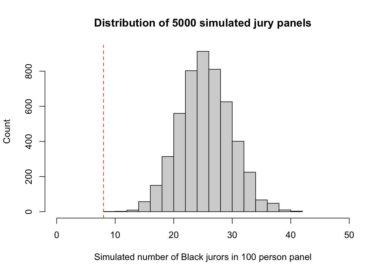
histogram ofpanels- how does this compare to the observation of \(x=8\)?
2.3 Using a binomial distribution
A different (and simpler) way of viewing this problem is to recognise that we have all of the conditions for a binomial distribution here. If we let the number of Black jurors on the 100-person panel be \(X\), then if we’re sampling independently and randomly with fixed \(p=0.26\), then we should have that \(X\sim\text{Bin}(100, 0.26)\).
As you might expect from statistical software, R can directly generate random numbers from common distributions such as the binomial.
The rbinom function allows us to generate random
observations from a binomial distribution. Its syntax is
rbinom(n, size, prob)
The arguments to this function are:
n- how many random numbers to generate. Note this is not the binomial sample size parameter \(n\)!size- the \(n\) parameter of the binomial distribution to useprob- the probability of success \(p\).
- How would you use the
rbinomfunction to simulate \(X\), the number of Black jurors in a jury panel of 100 individuals? - How would you modify your code to simulate 5000 values of \(X\)?
2.4 Exploring the results
We’ve now randomly simulated a large number of potential jury panels
consistent with this area in Alabama. Let’s do a little statistical
analysis on our results. You can use either the results from your own
function or rbinom - it shouldn’t matter which.
- Compute the
meanandvariance of your simulated \(X\)s. - If \(X\sim Bin(100,0.26)\) what are the theoretical mean and variance of \(X\)? Do these values agree with your simulations?
- Does the simulated distribution of \(X\) the values appear to be consistent with the observation \(x=8\)?
- What distribution would make a good approximation to that of \(X\)? Hint: we’re summing a large number of independent random variables.
- Re-draw/go back to your
histogram of the values of \(X\). Does the shape of the histogram agree with your expectation?
To control the ranges of the horizontal and vertical axes, we can add
the xlim and ylim arguments to our original
plotting command. To set the horixontal axis limits, we pass a vector of
two numbers to represent the lower and upper limits,
xlim = c(lower, upper), and repeat the same for
ylim to customise the vertical axis. For example,
plot(x=1:10, y=1:10, xlim=c(-10,10), ylim=c(0,20))
We don’t have to specify axis limits, and when omitted R will figure out something sensible for us.
- Re-draw your histogram using \(x\) axis limits that go from \(0\) up to \(50\).
It is often useful to add simple straight lines to lines to plots,
which can be achieved using the abline function.
abline can be used in three different ways:
- Draw a horizontal line: pass a value to the
hargument,abline(h=3)draws a horizontal line at \(y=3\) - Draw a vertical line: pass a value to the
vargument,abline(v=5)draws a vertical line at \(x=5\) - Draw a line with given intercept and slope: pass value to the
aandbarguments representing the intercept and slope respectively;abline(a=1,b=2)draws the line at \(y=1+2x\)
abline can be customised using any of the usual colour
and line modifications using colour (col), line types and
widths (lty, and
lwd).
- Add a vertical line at \(x=8\) to represent the observation in the Swain jury selection case.
- You can also customise your axis labels to be more readable - see the help for details.
- You can customise your line (and your histogram) using colour:
- Read the help page on using colour in plots and experiment with redrawing your hisorgram and vertical line using some custom colour.
- What do you conclude about the plausibility of observing \(x=8\) at random from this population?
You should end up with a plot that looks a little like this:
- Without using the normal distribution, how would you use your simulations to estimate \(P[X\leq 8]\)?
- Hints:
- Think about how you might determine how many of your simulated jury panels have 8 or fewer Black jurors?
- You can use the
<=operator to test every element of a vector. sumwill treat all the values ofTRUEin a vector as1andFALSEas0- You may need to make many more simulations to get a non-zero estimate.
- Ask for help if you’re stuck!
This is evidence that the model of random selection of the jurors in the panel is not consistent with the data from the panel. While it is possible that the panel could have been generated by chance, our simulation demonstrates that it is hugely unlikely.
The reality of the trial panel is very much at odds with the model’s assumption of random selection from the eligible population. When the data and a model are inconsistent, then the model is hard to justify. After all, the data are real but the model is just a set of assumptions. When assumptions are at odds with reality, we must question those assumptions.
Therefore the most reasonable conclusion is that the either the proportion of eligible Black jurors was far smaller than stated or the assumption of random selection is unjustified for this jury panel. As the proportion was not in doubt, the most reasonable conclusion is that the jury panel was not selected by random sampling from the population of eligible jurors. Notwithstanding the opinion of the Supreme Court, the difference between 26% and 8% is not so small as to be explained well by chance alone.
3 Further Exercises:
- How would you use the techniques above to simulate the selection (without replacement) of 10 trial jurors from the 100-person jury panel? Do your results indicate whether it is plausible to obtain no Black jurors purely at random?
- Link up your two simulations! First simulate the selection of a
representative 100-person panel using
rbinom, and then use your simulated panel tosamplea simulated trial jury without replacement. Revisit your analysis to see whether this affects your conclusions.