Practical 1-3: Likelihood Inference
We have seen in lectures that the MLEs for the parameters of several common distributions can be found in closed form. However, in general, the problem is not guaranteed to be so easy with a simple closed-form result. Therefore, in these situations, we will have to find and maximise the likelihood numerically.
For this practical, we will focus on the Poisson distribution, which is particularly appropriate for counts of events occuring randomly in time or space. While we can find a tidy mathematical result for this case, we’ll use it to illustrate the general method of maximum likelihood. Suppose we have a simple problem with one piece of data, \(X\), and we know that \(X\sim\text{Po}(\lambda)\) for some unknown parameter value \(\lambda\).
- Download the R Script - Right click, and Save As
- You will need the following skills from previous practicals:
- Basic R skills with arithmetic, functions, etc
- Manipulating and creating vectors:
c,seq, - Calculating data summaries:
mean,sum,length - Writing custom
functions - Drawing a histogram with
hist, and adding simple lines to plotsabline - Customising plots using
colour
- New R techniques:
- Drawing a plot of a simple function using
curve - Optimising a function with
optim - Extracting named elements of a list using the
$operator
- Drawing a plot of a simple function using
1 The Poisson Likelihood
Our likelihood calculations begin with writing down the likelihood function of our data. For a single observation \(X=x\) from a Poisson distribution, the likelihood is the the probability of observing \(X=x\) written as a function of the parameter \(\lambda\): \[ \ell(\lambda) = \mathbb{P}[X=x~|~\lambda] = \frac{e^{-\lambda}\lambda^x}{x!}. \]
To begin with, suppose we observe a count of \(X=5\).
- Write a simple function called
poissonthat takes argumentslambdawhich evaluates the Poisson probability \(\mathbb{P}[X=5~|~\lambda]\). Hint: You will need theexpandfactorialfunctions. - Evaluate the Poisson probability for \(X=5\) when \(\lambda=7\) - you should get a value of
0.1277167.
What we have just created is the likelihood function, \(\ell(\lambda)\), for the Poisson parameter \(\lambda\) given a single observation of \(X=5\).
Before we consider a larger data problem, let’s briefly explore this simplest case of a Poisson likelihood. Let’s begin with a plot of the likelihood function itself.
Using curve to plot a funtion
Given an expression for a function \(f(x)\), we can plot the values of \(f\) for various values of \(x\) in a given range. This can be
accomplished using an R function called curve. The main
syntax for curve is as follows:
curve(expr, from = NULL, to = NULL, add = FALSE,...)
The arguments are:
expr: an expression or function in a variablexwhich evaluates to the function to be drawn. Examples includesin(x)orx+3*x^2from,to: specifies the range ofxfor which the function will be plottedadd: ifTRUEthe graph will be added to an existing plot; ifFALSEa new plot will be created...: any of the standard plot customisation arguments can be given here (e.g.colfor colour,ltyfor line type,lwdfor line width)
For example, the following code when evaluated produces the plot below:
curve(x^3 - 5*x, from = -4, to = 4)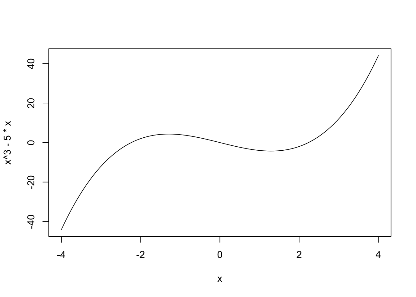
- Try out using
curveto draw a quick plot of the following functions:- \(f(x)=3x^2+x\) over \([0,10]\)
- \(f(x)=sin(x)+cos(x)\) over \([0,2\pi]\) as a blue curve. Note: R defines
pias the constant \(\pi\) - Use the
add=TRUEoption to superimpose \(g(x)=0.5sin(x)+cos(x)\) as a red curve over \([0,2\pi]\) on the previous plot.
- Now, use
curveand yourpoissonfunction to draw a plot of your Poisson likelihood for \(\lambda\in[0.1, 20]\). - By eye, what is the value \(\hat{\lambda}\) of \(\lambda\) which maximises the likelihood?
Typically, we usually work with the log-likelihood \(\mathcal{L}(\lambda)=\log\ell(\lambda)\), rather than the likelihood itself. This can often make the mathematical maximisation simpler, the numerical computations more stable, and it is also intrinsically connected to the idea of information and variance (which we will consider later).
- Modify your
poissonfunction to compute the logarithm of the Poisson probability, and call this new functionlogPoisson. You will need to use thelogfunction. - Re-draw the plot to show the log-likelihood against \(\lambda\). Do you find the same maximum value \(\widehat{\lambda}\)?
2 Likelihood methods for real data
The Poisson distribution has been used by traffic engineers as a model for light traffic as the Poisson is suitable for representing counts of independent events which occur randomly in space or time with a fixed rate of occurrence. This assumption is based on the rationale that if the rate of occurrence is approximately constant and the traffic is light (so the individual cars move independently of each other), then the distribution of counts of cars in a given time interval or space area should be nearly Poisson (Gerlough and Schuhl 1955).
For this problem, we will consider the number of right turns made at a specific junction during three hundred 3-minute intervals. The following table summarises these observations.| N | 0 | 1 | 2 | 3 | 4 | 5 | 6 | 7 | 8 | 9 | 10 | 11 | 12 |
| Frequency | 14 | 30 | 36 | 68 | 43 | 43 | 30 | 14 | 10 | 6 | 4 | 1 | 1 |
traffic <- rep(0:12, c(14,30,36,68,43,43,30,14,10,6,4,1,1))Note that we interpret these data as 14 observations of the value \(0\), 30 observations of the value \(1\), and so forth.
- Evaluate the piece of code above to create the vector
trafficcorresponding to the above data set. - Plot a
histogram of the data. Does an assumption of a Poisson distribution appear reasonable?
If we suppose a Poisson distribution might be a good choice of distribution for this dataset, we still need to find out which particular Poisson distribution is best by estimating the parameter \(\lambda\).
Let’s begin by constructing the likelihood and log-likelihood functions for this data set of 300 observations. Assuming that the observations \(x_1, \dots, x_{300}\) can be treated as 300 i.i.d. values from \(\text{Po}(\lambda)\), the log-likelihood function for the entire sample is: \[ \mathcal{L}(\lambda) = -n\lambda +\left(\sum_{i=1}^n x_i \right) \log \lambda, \] up to an additive constant from the factorial terms (which we know we can ignore for the purposes of these calculations).
- Write a new functions
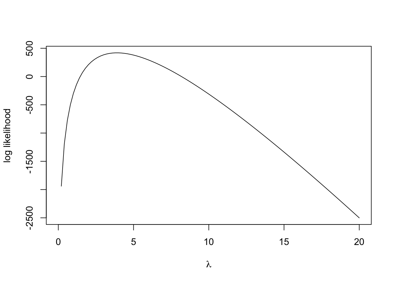
logLikewith a single parameterlambda, which evaluates the log-likelihood expression above for thetrafficdata and the supplied values oflambda. Hint: Uselengthandsumto compute the summary statistics. - Plot the log-likelihood against \(\lambda\) using
curve. Without further calculations, use the plot to have a guess at the maximum likelihood estimate \(\widehat{\lambda}\) – we’ll check this later!
2.1 Maximising the likelihood
The maximum likelihood estimate (MLE) \(\widehat{\lambda}\) for the \(\lambda\) parameter of the Poisson distribution is the value of \(\lambda\) which maximises the likelihood \[ \widehat{\lambda}=\operatorname{argmax}_{\lambda\in\Omega} \ell(\lambda)= \operatorname{argmax}_{\lambda\in\Omega} \mathcal{L}(\lambda). \]
Therefore to find the MLE, we must maximise \(\ell\) or \(\mathcal{L}\). We know we can do this
analytically for certain common distributions, but in general we’ll have
to optimise the function numerically instead. For such problems,
R provides various functions to perform a numerical
optimisation of a give function (even one we have defined ourself). The
function we will focus on is optim:
R offers several optimisation functions, however the one
we shall be using today is optim which is one of the most
general optimisation functions. This generality comes at the price of
having a lot of optional parameters that need to be specified.
For our purposes, we’re doing a 1-dimensional optimisation of a given
function named logLike. So the syntax we will use to
maximise this function is as follows
optim(start, logLike, lower=lwr, upper=upr, method='Brent', control=list(fnscale=-1))
The arguments are:
start: an initial value for \(\lambda\) at which to start the optimisation. Replace this with a sensible value.logLike: this is the function we’re optimising. In general, we can replace this with any other function.lower=lwr, upper=upr: lower and upper bounds to our search for \(\widehat{\lambda}\). Replacelwranduprwith appropriate numerical values; an obvious choice for this problem is the min and max of our data.method='Brent': this selects an appropriate optimisation algorithm for a 1-D optimisation between specified bounds. Other options are available for other classes of optimisation problem.control=list(fnscale=-1): this looks rather strange, but is simply tellingoptimto maximise the given function, rather than minimise which is the default (it’s instructing R to scale the function by a factor of \(-1\) and minimise the result).
optim returns a number of values in the form of a list.
The relevant components are:
par: the optimal value of the parametervalue: the optimum of the function being optimised.convergence: if0this indicates that the optimisation has completed successfully.
- Use
optimto maximise thelogLikefunction. You should choose an appropriate initial value for \(\lambda\), as well as sensibleupperandlowerbounds. - What value of \(\widehat{\lambda}\) do you obtain? How does this compare to your guess at the MLE?
- We know from lectures that the \(\widehat{\lambda}=\bar{X}\) – evaluate the
sample mean of the
trafficdata. Does this agree with your results from directly maximising the log-likelihood?
You should see output something like this:
## $par
## [1] 3.893333
##
## $value
## [1] 419.6223
##
## $counts
## function gradient
##       NA       NA
##
## $convergence
## [1] 0
##
## $message
## NULL
The output of optim is in the form of a
list. Unlike vectors, lists can combine many
different variables together (numbers, strings, matrices, etc) and each
element of a list can be given a name to make it easier to access.
For example, we can create our own lists using the list
function:
test <- list(Name='Donald', IQ=-10, Vegetable='Potato')
Once created, we can access the named elements of the list using the
$ operator. For example,
test$IQ
will return the value saved to IQ in the list,
i.e. -10. RStudio will show auto-complete suggestions for
the elements of the list after you press $, which can help
make life easier.
We can use this $ operator to extract the MLE value from
optim by first saving the results to a variable, called
results say, and then extracting the list element named
par, which corresponds to the maximising value of \(\lambda\).
- Extract the optimal value of \(\lambda\) from the output of
optimand save it to a new variable calledmle. - Re-draw your plot of the log-likelihood function, and use
ablineto:- Add a red solid vertical line at \(\lambda=\widehat{\lambda}\). Hint:
pass the
col='red'argument to your plotting function. - Add a blue dashed vertical line at \(\lambda=\bar{x}\).
- Add a red solid vertical line at \(\lambda=\widehat{\lambda}\). Hint:
pass the
- Do the results agree with each other, and with your guess at \(\widehat{\lambda}\)?
Let’s return to the original distribution of the data. The results of our log-likelihood analysis suggest that a Poisson distribution with parameter \(\widehat{\lambda}\) is the best choice of Poisson distributions for this data set.
- Re-draw the
histogram of thetrafficdata. - Modify your
poissonfunction to evaluate the Poisson probability \(\mathbb{P}[X=x]\) when \(X\sim\text{Po}(\widehat{\lambda})\). Save the function aspoissonProb. - The expected number of Poisson counts under this \(\text{Po}(\widehat{\lambda})\) distribution
will be \(300\times\mathbb{P}[X=x]\),
for \(x=0,\dots,16\). Use the
curvefunction toadddraw this function over your histogram in red. (We will ignore the fact that \(X\) is discrete for the time-being.) - Does this look like a good fit to the data?
We will return to the question of fitting distributions to data and the “goodness of fit” later next term.
2.2 Information and inference
For an iid sample \(X_1,\dots,X_n\) from a sufficiently nicely-behaved (“regular”) density function \(f(x_i~|~\theta)\) with unknown parameter \(\theta\), the sampling distribution of the MLE \(\widehat{\theta}\) is such that \[ \widehat{\theta} \rightsquigarrow \text{N}\left(\theta, \frac{1}{\mathcal{I}_n(\theta)}\right), \] as \(n \rightarrow\infty\). For large samples, we can also replace the expected Fisher information in the variance with the observed information, \(I(\hat{\theta})=-\mathcal{L}''(\widehat{\theta})\) instead, Whilst we may be used to finding Normal distributions in unusual places, this result is noteworthy as we never assumed any particular distribution of our data here. This result therefore provides us with a general method for making inferences about parameters of distributions and their MLEs for problems involving large samples!
In particular, we can apply this to our Poisson data problem above to construct a large-sample approximate \(100(1-\alpha)\%\) confidence interval for \(\lambda\) in the form: \[ \widehat{\lambda} \pm z^*_{\alpha/2} \frac{1}{\sqrt{-\mathcal{L}''(\widehat{\lambda})}}, \] where \(z^*_{\alpha/2}\) is the \(\alpha/2\) critical value of a standard Normal distribution and we have estimated the expected Fisher information \(\mathcal{I}_n(\theta)\) by the observed information \(I(\widehat{\lambda})=-\mathcal{L}''(\widehat{\lambda})\).
- We can request that
Rcomputes the second derivative at the maximum, \(\mathcal{L}''(\widehat{\lambda})\), as part of the maximisation process. To do this, re-run your optimisation, but add the additional argumenthessian=TRUE.
You should now obtain R output that looks like this:
## $par
## [1] 3.893333
##
## $value
## [1] 419.6223
##
## $counts
## function gradient
##       NA       NA
##
## $convergence
## [1] 0
##
## $message
## NULL
##
## $hessian
##           [,1]
## [1,] -77.05481- The output from
optimwill now contain an additional element namedhessian. Extract this element, multiply by -1, and save it asobsInfo. - To get the variance of \(\widehat{\lambda}\) we need to invert the
information matrix. We can achieve this using R’s
solvefunction. Try this now onobsInfo. Save this tovarMLE. - As
obsInfois just a scalar (or a \(1\times1\) matrix), we should just return the reciprocal \(\frac{1}{I(\widehat{\lambda})}\) - check this now! - Finally,
varMLEwill be in the form of a \(1\times 1\) matrix rather than a scalar (as the Hessian matrix is a matrix of the second order partial derivatives). To extract the value from within the matrix, run the following codevarMLE <- varMLE[1,1]
- Use your standard Normal tables (or R’s built-in function
qnorm) to find the critical \(z^*_{\alpha/2}\) value for a 95% confidence interval. Save this aszcrit. - Combine
mle,zcrit, andvarMLEto evaluate an approximate 95% Wald confidence interval for \(\lambda\). - Return (and possibly re-draw) the plot of your log-likelihood function, with the MLE indicated as a vertical line. Add the limits of the confidence interval to your plot as vertical green lines.
- What does the confidence interval suggest about the reliability of your estimate.
- Does the log-likelihood look reasonably quadratic near the MLE? Does this affect your conclusions, and how would you investigate this further?