Practical 2-3: Bayesian Hypothesis Testing
In this practical we will experiment with the exponential distribution which is commonly used to model the time to the occurrence of some event. Such events may be death of a person, failure of a piece of equipment, development of (or remission) of symptoms, health code violation (or compliance) etc. The times to the occurrences of events are known as “lifetimes” or “survival times” or “failure times” according to the event of interest in the fields of study.
- Download the R Script - right click, and Save As
- You will need the following skills from previous practicals:
- Basic R skills with arithmetic, functions, etc
- Manipulating and creating vectors:
c,seq,length - Plotting a scatterplot with
plot - Use of the
whichcommand.
- New R techniques:
- Using the
dexpandgammafunctions. - Using
functionwith multiple arguments as input.
- Using the
1 The data
This is a part of a data set of waiting times (in minutes) before service of 30 Bank customers and examined and analyzed by Ghitany et al. (Lindley distribution and its application, Mathematics and Computers in Simulations, 2008).
| Times | 0.8 | 0.8 | 1.3 | 1.5 | 1.8 | 1.9 | 1.9 | 2.1 | 2.6 | 2.7 |
| Times | 2.9 | 3.1 | 3.2 | 3.3 | 3.5 | 3.6 | 4.0 | 4.1 | 4.2 | 4.2 |
| Times | 4.3 | 4.3 | 4.4 | 4.4 | 4.6 | 4.7 | 4.7 | 4.8 | 4.9 | 4.9 |
As usual, we begin in R by entering the data and examining summaries of the data, and plots of the data, initially.
x = c(0.8, 0.8, 1.3, 1.5, 1.8, 1.9, 1.9, 2.1, 2.6, 2.7, 2.9, 3.1, 3.2, 3.3, 3.5, 3.6, 4.0, 4.1, 4.2, 4.2, 4.3, 4.3, 4.4, 4.4, 4.6, 4.7, 4.7, 4.8, 4.9, 4.9)
summary(x)
## Min. 1st Qu. Median Mean 3rd Qu. Max.
## 0.800 2.225 3.550 3.317 4.375 4.900sd(x)## [1] 1.295638hist(x, col = 2, main = 'Waiting times (minutes) in banks')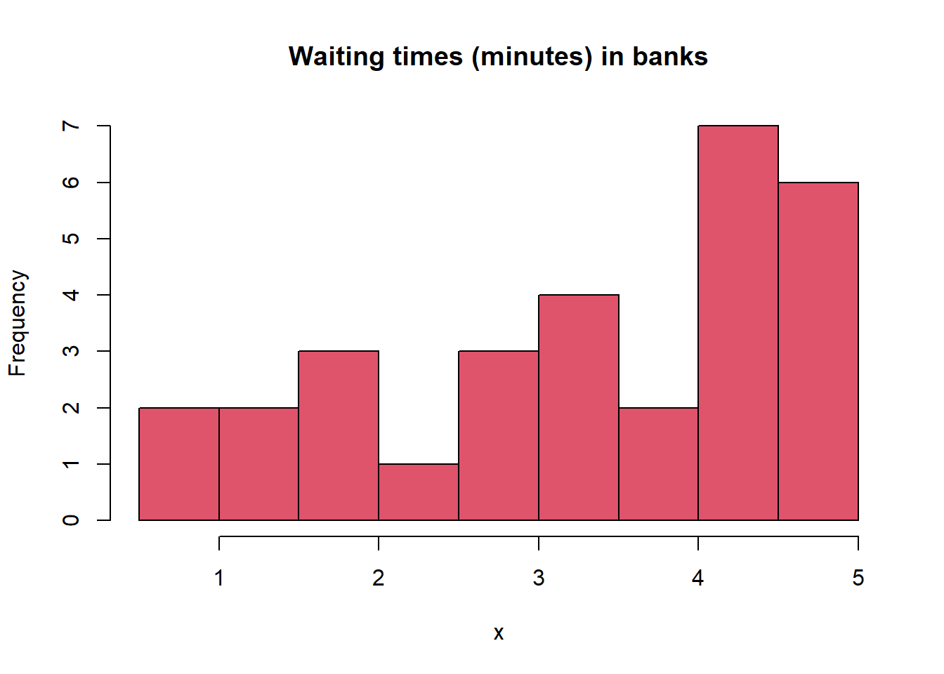
2 Theory reminder.
The exponential distribution as a likelihood. The pdf of the exponential distribution is \[ f(x|\lambda) = \lambda e^{-\lambda x} \]
for \(\lambda >0\) and \(x\in[0,\infty)\).The Bayes factor for simple vs. simple hypotheses. As we have seen, for these simple tests finding the Bayes factor \(B_{01}\) in favour of \(H_0\) against \(H_1\) reduces to computing the likelihood ratio. Then finding posterior probabilities also becomes easy as we have the formula. So in the particular case of the exponential we have that the Bayes factor of \(H_0: \lambda = \lambda_0\) vs. \(H_1: \lambda = \lambda_1\) is simply \[ B_{01} = \left(\frac{\lambda_0}{\lambda_1}\right)^n e^{-(\lambda_0-\lambda_1)\sum_{i=1}^nx_i} \] You can check this by yourself later for practice. So, it easy to derive the Bayes factor and then we can also derive posterior probabilities from \[ p_0 = \left[1+\frac{\pi_1}{\pi_0}B_{01}^{-1}\right]^{-1}, \] which of course depends on the prior probabilities.
The gamma distribution as a conjugate likelihood. As we know the conjugate prior for an expontial \(x\) is the gamma distribution: \[ f(\lambda) = \frac{\beta^\alpha}{\Gamma(\alpha)}\lambda^{\alpha-1} e^{-\beta \lambda} \]
3 Applying simple vs. simple tests to the data.
Assume that for the given data we have a suspicion that parameter \(\lambda\) is concentrated somewhere within the region \([0,1]\).- Assume that, initially, test the hypothesis \(H_0: \lambda = 0.5\) vs. \(H_0: \lambda = 0.6\). Define appropriately
named objects for the quantities that you will use:
l0,l1for the prior hypotheses,nfor sample size, andSfor the sum of the data. - What are the results in terms of \(B_{01}\), \(2log B_{10}\)? Calculate the posterior probabilities \(p_0\), \(p_1\), assuming that the two hypotheses are equally likely a-priori. What are your conclusions?
Of course, in this simple case we can “cheat” a bit, and use the
build-in R function dexp for calculating the ratio. Type
`?dexp’ to see how this function works.
- Repeat the previous calculations for \(B_{01}\), \(2log
B_{10}\) using
dexp(type?dexp) and taking the product of the result via functionprod. - Check whether the results are in agreement.
It would be desirable to perform multiple comparisons in the region \([0,1]\) under the alternative. However, repeating the above procedure for various values of \(\lambda_1\) is not convenient based on the previous approach. For this reason we will first define our own function in R.
- Based on your previous code, from Exercise 3.1, define a function
fwith argumentsdata,l0andl1that can be used for any given data and set of point hypotheses. The function should provide as end result \(2\log B_{10}\). - Compare with the previous result for the same set of hypotheses to check whether there is agreement.
data and
l0 and use the command seq for defining a grid
of values for the argument l1.- Type
?seqto remember how to use this command. Then define an objectgrid1based onseqwhich will be an equally spaced grid of 100 values from 0 to 1. - Storing results to an object
logB10, usegridl1as input to your functionfusing the samedataandl0as before. - Assuming that we would be strict and reject \(H_0\) if \(2\log
B_{10} >1\) find the minimum and the maximum \(\lambda_1\)s for which we would reject.
Store them to objects
minl1andmaxl1, respectively. Hint: You can use thewhich, command which we used in the previous practicals.
- Plot the results having on the x-axis the sequence of \(\lambda_1\) values and on the y-axis the calculated \(2\log B_{10}\).
- Use the command
ablineto highlight horizontally where \(2\log B_{10} >1\) and vertically the minimum and maximum \(\lambda_1\)s as the boundaries where this happens.
- What are your conclusions from the plot?
4 Theory reminder.
The Bayes factor for simple vs. composite hypotheses. As we have seen (or will see), for these type of tests the Bayes factor is given by \[ B_{01} = \frac{f(x|\theta=\theta_0)}{\int_{\theta\in\Omega} f(x|\theta)f(\theta)\mathrm{d}\theta}. \]
The gamma distribution as a conjugate prior. As we know the conjugate prior for the exponential is the gamma distribution: \[ f(\lambda) = \frac{\beta^\alpha}{\Gamma(\alpha)}\lambda^{\alpha-1} e^{-\beta \lambda}. \]
The Bayes factor of the Exponential-Gamma model. It can be shown with some mathematical derivations that the resulting Bayes factor for our model in the simple vs. composite case is given by \[ B_{01} = \frac{\lambda_0^n \Gamma(\alpha)(\sum_i x_i + \beta)^{n+\alpha}}{e^{\lambda_0\sum_i x_i}\Gamma(n+\alpha)\beta^\alpha}. \]
5 Applying simple vs. composite tests to the data.
Assume that we make the prior assumption that \(\alpha =2\) and \(\beta=4\).- This time create a function
f2that takes as inputdata,l0,alphaandbetaand gives as output the posterior probability of \(H_0\) (use the formula shown in Section 2). Use thegammafunction (type?gamma) - Apply the function to the dataset assuming this time that
l0=0.3. - If you have coded this correctly you will an output approximately equal to 0.836. What can we say based on the output?
- Create a function
f3that takes as further input the additional argumentpi0for the prior probability of \(H_0\) and produces again as output the posterior probability of \(H_0\). - Assume that for some reason we believe that \(H_0\) is more likely and assign the prior
odds to be equal to 2.333333. Use your function
f3to find the posterior probability of the null. - Has the posterior probability increaed or decreased, and is the result expected?
Under the assumption \(\alpha =2\), \(\beta=4\), we essentially “centered” the prior around the \(H_0\), because the prior expectation and variance from the gamma prior are given by \[ E(\lambda) = \frac{\alpha}{\beta}=\frac{2}{4}=0.5, ~~ Var(\lambda) = \frac{\alpha}{\beta^2}=\frac{2}{16}=0.125. \]
- Think of values of \(\alpha\) and \(\beta\) that give again a prior expectation equal to 0.5, but that result in a higher prior variance.
- Apply then your function
f1using these hyperparameters. - What is the resulting posterior probability now, and how do you explain the change in comparison to the result in Exercise 5.1?