4 Solving linear PDEs via eigenfunction expansions – MATH 2811 Mathematical Methods II Weeks 6-10

4.1 A general linear PDE model

Chapters 1–3 developed the ingredients we need: mode expansions, spatial eigenvalue problems, and the general theory of boundary-value problems. In this chapter we put those ideas to work.

Our prototype is a broad class of linear PDE models of the form \[ \ddy{u}{t} = L u + h(x,t). \tag{4.1}\] Here we consider a one-dimensional model of a scalar function \(u(x,t)\) on a domain \(x \in[a,b]\) and \(t>0\). There are several ingredients to specify:

The central idea of this chapter is:

\[ \boxed{ \text{the spatial eigenproblem determines the modes,} }\Rightarrow \] \[ \boxed{ \text{the rest of the PDE determines what those modes do.} } \]

4.1.1 The operator

The operator \(L\) is a linear operator, satisfying \[ L[a\,u_1 + b\,u_2] = a\,Lu_1 +b\,Lu_2. \] If it has derivatives they are only in the spatial variable \(x\). It can represent the spreading, transport and creation/destruction of the scalar \(u\).

Examples The diffusion operator: \[ L = \pder{}{x}{2} \Rightarrow \ddy{u}{t} = \pder{u}{x}{2} + h(x,t) \] or \[ L = \pder{}{x}{2} + v\ddy{}{x} + \mu \Rightarrow \ddy{u}{t} = \pder{u}{x}{2} + v\ddy{u}{x} +\mu u + h(x,t) \] which is a model with a density \(u\) diffusing, maybe the density of a dissolved drug. The term \(v\ddy{}{x}\) could represent a fluid flow, maybe blood moving the drug density at a speed \(v\). Finally, the term \(\mu u\) could represent the degradation/creation of the drug at a rate \(\mu\) (maybe enzyme action).

We can use much more elaborate choices of \(L\); for what follows, the crucial requirement is linearity.

4.1.2 The “source/forcing” term \(h(x,t)\)

The function \(h(x,t)\), sometimes referred to as a forcing term, does not depend on the value of \(u\), so provides some external (to the system) change in the rate of production/loss of \(u\) (which is what \(\ddy{u}{t}\) represents).

If \(u\) were representing a population, it could represent immigration/migration, or in the diffusing drug example discussed above it could be an intravenous flow.

An example \[ h(x,t) = \sin\left(\pi\frac{x-a}{b-a}\right)\cos(\omega t). \] This provides a forcing which is zero at the boundaries, and maximal in the middle of the domain. It varies from increasing \(u\) when \(\cos(\omega t)>0\), to decreasing \(u\) when \(\cos(\omega t)<0\), a change which oscillates at a rate \(\omega\).

A rather famous forcing term!

In September 2026, OpenAI announced a construction of a finite-time singularity in the three-dimensional Navier–Stokes equations, one of the Clay Millennium Prize Problems.

A central feature is that the fluid starts at rest and is acted upon by a smooth external force. The force itself does not become infinite, but the resulting fluid velocity develops a singularity in finite time.

The Navier–Stokes equations are nonlinear and considerably more complicated than our linear prototype, but they illustrate an important point: specifying the forcing is part of specifying the physical and mathematical problem.

The distinction between a forced and an unforced PDE can matter enormously!

If \(h(x,t)=0\) then the evolution equation is referred to as homogeneous. If it is non-zero the evolution equation is referred to as inhomogeneous. This is separate from whether the boundary or initial data are homogeneous.

Inhomogeneous-homogeneous decomposition

For every inhomogeneous evolution equation, there is an associated homogeneous equation obtained by setting \(h(x,t)=0\). If \(u_p\) is one particular solution of the inhomogeneous equation and \(u_h\) is any solution of the corresponding homogeneous equation, then \[ u=u_p+u_h \] is also a solution of the inhomogeneous differential equation, by linearity. To preserve specified boundary or initial data, the added homogeneous solution must satisfy the corresponding homogeneous data.

4.1.3 Boundary conditions

To make our problem concrete we need to supply \(p\) boundary conditions, with \(p\) matching the spatial order of the operator, i.e. we would need two boundary conditions in the examples above. It is useful to write these abstractly as \[ BC_i[u]=\gamma_i(t),\qquad i=1,\ldots,p, \] where the \(BC_i\) are linear boundary operators acting on the values of \(u\) and its derivatives at \(x=a,b\).

Examples: \[ BC_1[u] = \ddy{u}{x}{\Large\vert}_{x=a}=0, \qquad BC_2[u] = \ddy{u}{x}{\Large\vert}_{x=b}=0. \] But we could have more elaborate linear choices, for example \[ BC_1[u]=\ddy{u}{x}{\Large\vert}_{x=a}+5u(a,t)=0, \qquad BC_2[u]=u(a,t)+u(b,t)=10. \]

A reminder from chapter 1: A boundary condition is homogeneous when the right-hand side is zero, \(\gamma_i(t)=0\). Otherwise it is inhomogeneous.

So a condition such as \[ u(a,t)+5u_x(a,t)=0 \] is still homogeneous, even though neither term need vanish individually.

Hereafter, when the boundary conditions are homogeneous, we will simply write \(BC_i u=0\).

4.1.4 Initial conditions

Finally, this problem needs a start point, the initial condition. That is some value of the function \(u\) at \(t=0\): \[ u(x,0) = g(x). \]

4.1.5 Where does this model occur?

4.1.6 Some applied examples

This material is not examinable. It is here to show how widely the model \[ u_t=Lu+h \] appears in applied mathematics.

Surface flux transport

The equation

\[ \ddy{u}{t} = D\nabla^2 u -\nabla\cdot\left({\mathbfit{v}}u\right) +h(\mathbfit{x},t) \]

is used to model the line-of-sight component of the Sun’s magnetic field at its surface. This is technically a two-dimensional version of our model, but it has exactly the same basic structure.

The field diffuses due to convective motion at the Sun’s surface. The velocity \(\mathbfit{v}\) represents large-scale motions such as differential rotation and meridional circulation. The source term \(h\) is particularly important: it represents the emergence of new, strong, localised magnetic field in active regions.

Linear reaction–diffusion systems

A coupled system can take the form

\[\begin{align} \ddy{u}{t} &= D_1\nabla^2u+f_1u+f_2v,\\ \ddy{v}{t} &= D_2\nabla^2v+g_1u+g_2v, \end{align}\]

with \(D_1,D_2,f_1,f_2,g_1,g_2\) constants. This can arise by linearising a nonlinear reaction–diffusion system,

\[\begin{align} \ddy{u}{t} &= \nabla^2u+f(u,v),\\ \ddy{v}{t} &= \nabla^2v+g(u,v). \end{align}\]

Turing famously used this type of linearisation to study the formation of spatial patterns such as spots and stripes.

One of the striking lessons is that the linearised modes can successfully predict important features of the much more complicated nonlinear dynamics.

Some familiar spatial eigenproblems

Not every equation we have met is itself a time-dependent PDE of the form \(u_t=Lu+h\). Some instead arise as the spatial eigenvalue problems used inside that PDE method.

For example, the Bessel equation

\[ x^2y''+xy'+(x^2-\nu^2)y=0 \]

appears naturally in radial problems in polar and cylindrical coordinates, as we saw in Chapter 2.

Similarly, the Chebyshev equation

\[ (1-x^2)y''-xy'+n^2y=0 \]

generates the Chebyshev polynomials, which are widely used in approximation and spectral methods.

These examples are useful reminders that the spatial basis need not be Fourier modes.

4.2 Solving the model by eigenfunction expansion

The solution strategy is now almost forced upon us by Chapters 1–3:

find the spatial eigenfunctions of \(L\) with the required boundary conditions;
expand both the solution and forcing in those modes;
use the eigenvalue relation to reduce the PDE to equations for the modal amplitudes.

Let us carry this out.

For the one-dimensional problems considered here, we assume that the spatial eigenproblem has the Sturm–Liouville structure discussed in Chapter 3, or can be transformed into that form. We therefore have a suitable complete set of spatial eigenfunctions in which to expand the solution and forcing. For simplicity we write the eigenproblem here in the unweighted operator form \[ Ly_n=-\lambda_n y_n. \] If the Sturm–Liouville formulation contains a weight \(r(x)\), the weight appears explicitly in the coefficient projections, as in Chapter 3.

Let \(y_n(x)\) denote these eigenfunctions, with the required homogeneous boundary conditions. We expand the solution in this spatial eigenbasis: \[ u(x,t) = \sum_n c_n(t)y_n(x). \]

By the results of Chapters 1 and 3, the forcing can be decomposed in the same eigenbasis: \[ h(x,t) = \sum_n h_n(t)y_n(x). \] For a self-adjoint problem the \(h_n(t)\) are obtained by the usual weighted coefficient-grab formula. For a non-self-adjoint problem, Chapter 3 showed that the corresponding adjoint eigenfunctions are used to calculate these coefficients.

If we substitute this into our model we obtain

\[ \sum_n\ddt{c_n(t)}y_n(x) = \sum_n c_n(t)L y_n(x) +\sum_n h_n(t)y_n(x) \] (as \(L\) is a spatial variable operator only). The defining advantage of this basis is the eigen-equation \[ Ly_n(x)=-\lambda_n y_n(x), \] with \(\lambda_n\) constant. We can therefore bring the sums together mode by mode:

\[ \sum_n\left[\ddt{c_n(t)} +\lambda_n c_n(t) - h_n(t)\right]y_n(x) = 0. \] By uniqueness of the eigenfunction expansion (or equivalently by projecting onto each mode), each modal coefficient must vanish. That means we have to solve the following ordinary differential equations for each \(n\): \[ \ddt{c_n(t)} +\lambda_n c_n(t) - h_n(t) = 0. \] Remember, the only unknowns here are the functions \(c_n(t)\). If we can solve this ordinary differential equation for the \(c_n(t)\) then we have our solution to the original partial differential equation: \[ u(x,t) = \sum_n c_n(t)y_n(x). \] The good news is that we can, it’s just a first-order ODE. which can be solved by the integrating factor method. The solution is \[ c_n(t) = \mathrm{e}^{-\lambda_n t}\left( c_n(0) +\int_{0}^{t}\mathrm{e}^{\lambda_n t'}\,h_n(t')\,\mathrm{d}t'. \right). \tag{4.2}\]

The homogeneous solution in Equation 4.2 is: \[ a_n\mathrm{e}^{-\lambda_n t}. \] The inhomogeneous solution is: \[ \mathrm{e}^{-\lambda_n t}\int_{0}^{t}\mathrm{e}^{\lambda_n t'}h_n(t')\mathrm{d}t'. \]

The constants of integration are determined from the initial condition: \[ u(x,0) = \sum_n c_n(0)y_n(x) = g(x), \] and Chapter 1 tells us how to project \(g(x)\) onto the eigenbasis to determine the constants \(c_n(0)\). But what about the boundary conditions? Well, from linearity and the fact \(L\) is a spatial operator, we have, \[ BC_i u =\sum_n c_n(t)BC_i y_n = 0, \] so the functions \(y_n\) carry the homogeneous boundary conditions: \[ BC_i y_n =0. \] This is where linearity is important. If the original PDE has inhomogeneous boundary conditions, we first use the lifting idea from Chapter 3 to reduce them to homogeneous ones. If a function \(\ell(x,t)\) is chosen to carry the boundary data and we write \[ u=v+\ell, \] then \[ v_t=Lv+\big[h+L\ell-\ell_t\big], \qquad BC_i[v]=0. \] Thus the same eigenfunction method applies to \(v\), with a modified forcing term. If the boundary data are time-independent then \(\ell_t=0\).

Let’s summarise this.

The modal recipe

We have proposed that the solution to the problem \[ \ddy{u}{t} = L u + h(x,t), \] with \(p\) boundary conditions \[ BC_{i}[u]=0,\qquad i=1,\ldots,p, \] takes the form: \[ u(x,t) = \sum_n c_n(t)y_n(x), \] where the \(y_n\) satisfy the eigen-equation: \[ L y_n =-\lambda_n y_n, \] and each \(y_n\) satisfies the \(p\) boundary conditions: \[ BC_i y_n=0. \] Finally, the temporal functions \(c_n(t)\) take the form \[ c_n(t) = \mathrm{e}^{-\lambda_n t}\left( c_n(0) +\int_{0}^{t}\mathrm{e}^{\lambda_n t'}\,h_n(t')\,\mathrm{d}t' \right), \] where \[ h(x,t) = \sum_n h_n(t)y_n(x). \]

4.3 A concrete forced Fourier example

The general calculation is compact but abstract, so let us see it in the familiar Fourier setting.

If we choose the operators \[ L = \pder{}{x}{2},\quad BC_1[u] = \ddy{u}{x}{\Large\vert}_{x=a}\quad = BC_2[u] = \ddy{u}{x}{\Large\vert}_{x=b}=0, \] then the solution requires we solve the eigen-problem: \[ \deriv{y_n}{x}{2} = -\lambda_n y_n,\quad \dds{y_n}{x}{\Large\vert}_{x=a}=0,\quad \dds{y_n}{x}{\Large\vert}_{x=b}=0. \] Its solution is easily seen to be \[ y_n = \cos\left(\frac{n\pi(x-a)}{b-a}\right),\quad \lambda_n = \frac{n^2\pi^2}{(b-a)^2} \] for \(n=0,1,2,\ldots\).

The argument in the previous section states that the proposed solution to the PDE \[ \ddy{u}{t} = \deriv{u}{x}{2} + h(x,t), \] takes the form \[ u(x,t) = \sum_{n=0}^{\infty}c_n(t)\cos\left(\frac{n\pi(x-a)}{b-a}\right). \]

This is just a Fourier series. We know we can represent any reasonable forcing function \(h(x,t)\) using the standard formula \[ h(x,t) = \sum_{n=0}^{\infty}h_n(t) \cos\left(\frac{n\pi(x-a)}{b-a}\right),\quad h_n(t) = \frac{L}{b-a}\int_{a}^{b}h(x,t)\cos\left(\frac{n\pi(x-a)}{b-a}\right)\mathrm{d}x. \] The same is true of the initial condition: \[ g(x) = \sum_{n=0}^{\infty}c_n(0)\cos\left(\frac{n\pi(x-a)}{b-a}\right),\quad c_n(0) = \frac{l}{b-a}\int_{a}^{b}g(x)\cos\left(\frac{n\pi(x-a)}{b-a}\right)\mathrm{d}x, \] where \(l=2\) if \(n>0\) or \(l=1\) if \(n=0\). These expansions give us the values required to set the initial modal amplitudes \(c_n(0)\) in Equation 4.2.

The forcing \(h(x,t)\) likewise does not itself need to satisfy the same Neumann boundary conditions as \(u\).

So we can now set all our constants in the equation and we have a complete form for \(c_n(t)\).

A specific forcing

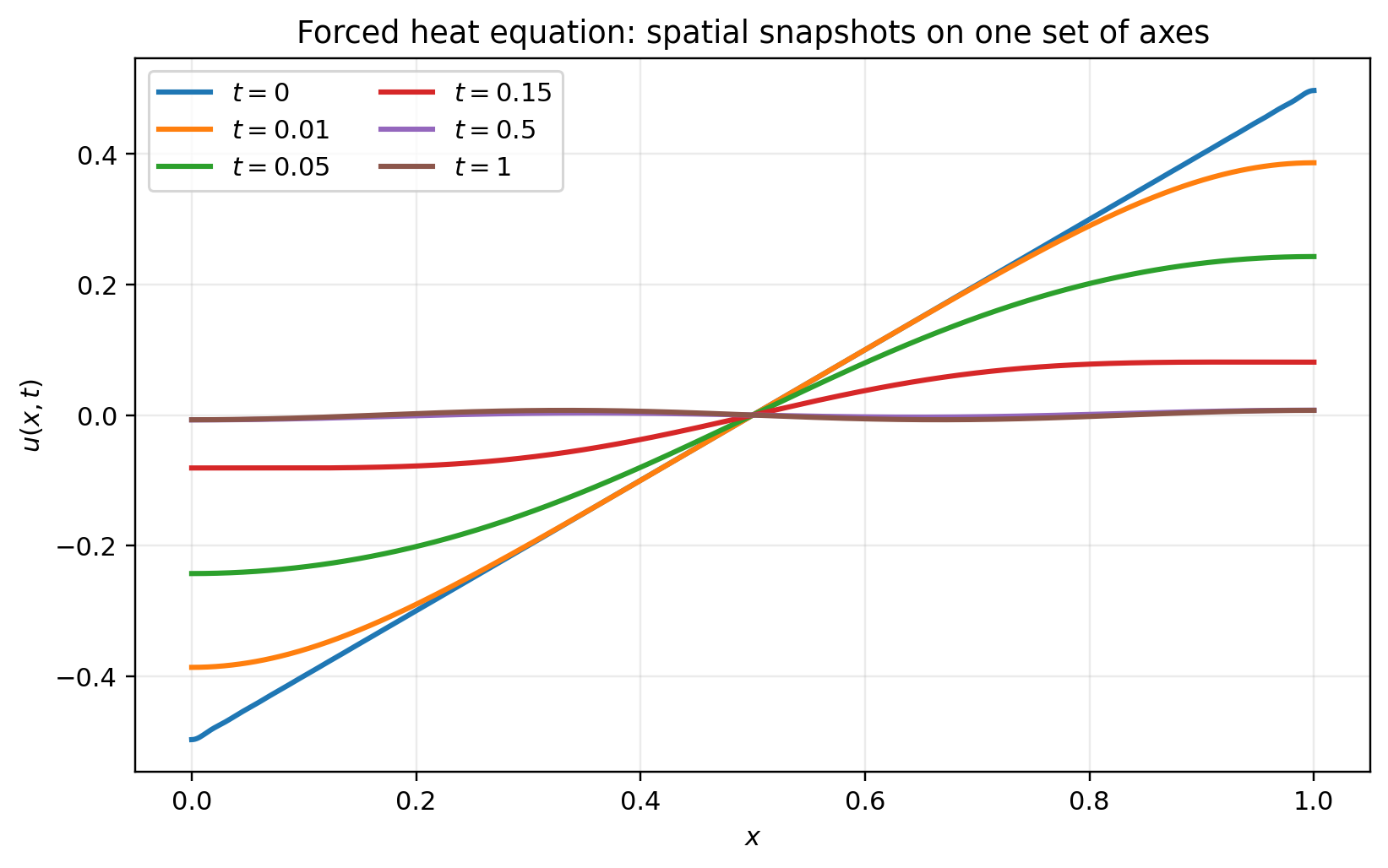
For example, if we make our lives simple and assume \(a=0,b=1\) and \[ h(x,t)=\sin(\omega t)\cos(3\pi x), \qquad g(x)=x-\frac12, \] then all \(h_n(t)=0\) except \[ h_3(t)=\sin(\omega t). \]

The initial coefficients are \[ c_n(0) = 2\int_0^1 \left(x-\frac12\right)\cos(n\pi x)\,\mathrm{d}x = \frac{2(\cos(n\pi)-1)}{n^2\pi^2}, \] for \(n>0\), with \(c_0(0)=0\).

Thus, if \(n\neq3\), \[ c_n(t)=c_n(0)\mathrm{e}^{-n^2\pi^2t}, \] so every unforced non-zero mode simply decays exponentially.

For the forced mode, let \[ \lambda_3=9\pi^2. \] Then \[ c_3'(t)+\lambda_3c_3(t)=\sin(\omega t), \] and hence \[ c_3(t) = \mathrm{e}^{-\lambda_3t} \left[ c_3(0)+ \int_0^t \mathrm{e}^{\lambda_3s}\sin(\omega s)\,\mathrm{d}s \right]. \]

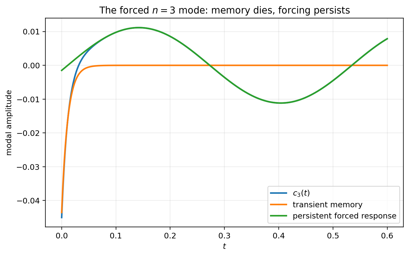
Evaluating the integral gives \[ \boxed{ c_3(t) = \left( c_3(0)+\frac{\omega}{\lambda_3^2+\omega^2} \right)\mathrm{e}^{-\lambda_3t} + \frac{ \lambda_3\sin(\omega t)-\omega\cos(\omega t) }{ \lambda_3^2+\omega^2 }. } \]

The first term is a transient and decays exponentially. The second is a persistent oscillation forced at frequency \(\omega\). Thus, for large \(t\), \[ c_3(t) \approx \frac{ \lambda_3\sin(\omega t)-\omega\cos(\omega t) }{ \lambda_3^2+\omega^2 }. \]

We see in Figure 4.1 (a) the decay from the linear initial condition to this trigonometric limiting behaviour.

So the forcing eventually dominates the \(\cos(3\pi x)\) mode, while the memory of the initial condition decays away. This is illustrated in Figure 4.1, panel (b).

Note the initial condition has essentially vanished from the long-time solution as the forcing takes over.

What made the calculation work?

The Fourier example used exactly the two ingredients developed in Chapter 3:

orthogonality, which lets us isolate individual modes;
a coefficient formula, which lets us expand the initial condition and forcing in the eigenbasis.

For Fourier modes these are the familiar sine and cosine coefficient formulae. For a more general operator \(L\), Chapter 3 showed how the same role is played by the eigenfunctions and, where necessary, their adjoint eigenfunctions.

So this example is not a special trick: it is a concrete instance of the general theory.

It is now time to try this out for yourselves.

Problem sheet 2 questions 1–3 contain similar examples which we will work through in class and tutorials.

4.4 Steady states: recovering \(Lu=f\)

The connection with Chapter 3 is immediate. If the system reaches a time-independent state, then \(u_t=0\) and \[ Lu+h(x)=0, \] or equivalently \[ \boxed{Lu=f(x),\qquad f=-h.} \] Thus the inhomogeneous boundary-value problem studied in Chapter 3 is exactly the equation for a steady state of our PDE model.

For a time-dependent solution we use the same spatial eigenfunctions, but allow their amplitudes to vary with time: \[ u(x,t)=\sum_n c_n(t)y_n(x). \] The spatial mathematics is therefore unchanged; what changes is that the modal coefficients satisfy ODEs rather than algebraic equations.

Example: Watching a PDE approach the solution we found in Chapter 3

Consider the forced heat equation

\[ \frac{\partial u}{\partial t} = \frac{\partial^2u}{\partial x^2}-x, \qquad 0<x<1, \]

with boundary conditions

\[ u(0,t)=u(1,t)=0, \]

and initial condition

\[ u(x,0)=0. \]

We start with a flat profile, continuously apply the forcing \(h(x)=-x\), and ask what happens as time passes.

Step 1: Calculate the equilibrium directly

If the system reaches a steady state \(u_s(x)\), then

\[ \frac{\partial u_s}{\partial t}=0, \]

so the PDE becomes

\[ u_s''=x, \qquad u_s(0)=u_s(1)=0. \]

Hang on – this is exactly the boundary-value problem we solved in Chapter 3!

Integrating twice,

\[ u_s(x)=\frac{x^3}{6}+Ax+B. \]

Applying the boundary conditions gives

\[ B=0,\qquad A=-\frac16, \]

and therefore

\[ u_s(x)=\frac{x^3-x}{6}. \]

That gives us a prediction for the final profile, without solving the time-dependent problem at all.

But does our time-dependent eigenfunction solution actually approach it?

Step 2: Solve the temporal system

The spatial eigenfunctions are

\[ y_n(x)=\sin(n\pi x), \qquad \lambda_n=n^2\pi^2, \qquad n=1,2,\ldots \]

We expand the solution as

\[ u(x,t)=\sum_{n=1}^{\infty}c_n(t)\sin(n\pi x). \]

The forcing coefficients are

\[ \begin{aligned} h_n &=2\int_0^1(-x)\sin(n\pi x)\,\mathrm{d}x\\ &=\frac{2(-1)^n}{n\pi}. \end{aligned} \]

So each temporal coefficient satisfies

\[ \frac{\mathrm{d}c_n}{\mathrm{d}t} +n^2\pi^2c_n = \frac{2(-1)^n}{n\pi}. \]

Our initial condition \(u(x,0)=0\) means that \(c_n(0)=0\) for every mode.

Using the temporal solution formula from earlier in this chapter gives

\[ c_n(t)= \frac{2(-1)^n}{n^3\pi^3} \left(1-\mathrm{e}^{-n^2\pi^2t}\right). \]

The full solution is therefore

\[ u(x,t)= \sum_{n=1}^{\infty} \frac{2(-1)^n}{n^3\pi^3} \left(1-\mathrm{e}^{-n^2\pi^2t}\right) \sin(n\pi x). \]

Step 3: What happens as time passes?

Every eigenvalue is positive, so

\[ \mathrm{e}^{-n^2\pi^2t}\longrightarrow0 \qquad\text{as }t\longrightarrow\infty. \]

Our solution approaches

\[ u(x,t)\longrightarrow \sum_{n=1}^{\infty} \frac{2(-1)^n}{n^3\pi^3}\sin(n\pi x). \]

But this is precisely the eigenfunction expansion we found in Chapter 3 for

\[ u_s''=x, \qquad u_s(0)=u_s(1)=0. \]

Thus

\[ \lim_{t\to\infty}u(x,t) = \frac{x^3-x}{6}. \]

The two approaches give the same answer!

So what have we gained by solving the time-dependent problem?

Chapter 3 told us what the equilibrium looks like. Chapter 4 tells us how the system approaches it.

Each mode has a transient contribution proportional to

\[ \mathrm{e}^{-n^2\pi^2t}, \]

which dies away as time passes. The higher-frequency modes decay more rapidly, while the forcing maintains the non-zero equilibrium profile.

The steady-state calculation and the time-dependent calculation are not competing methods: they answer different questions about the same system.

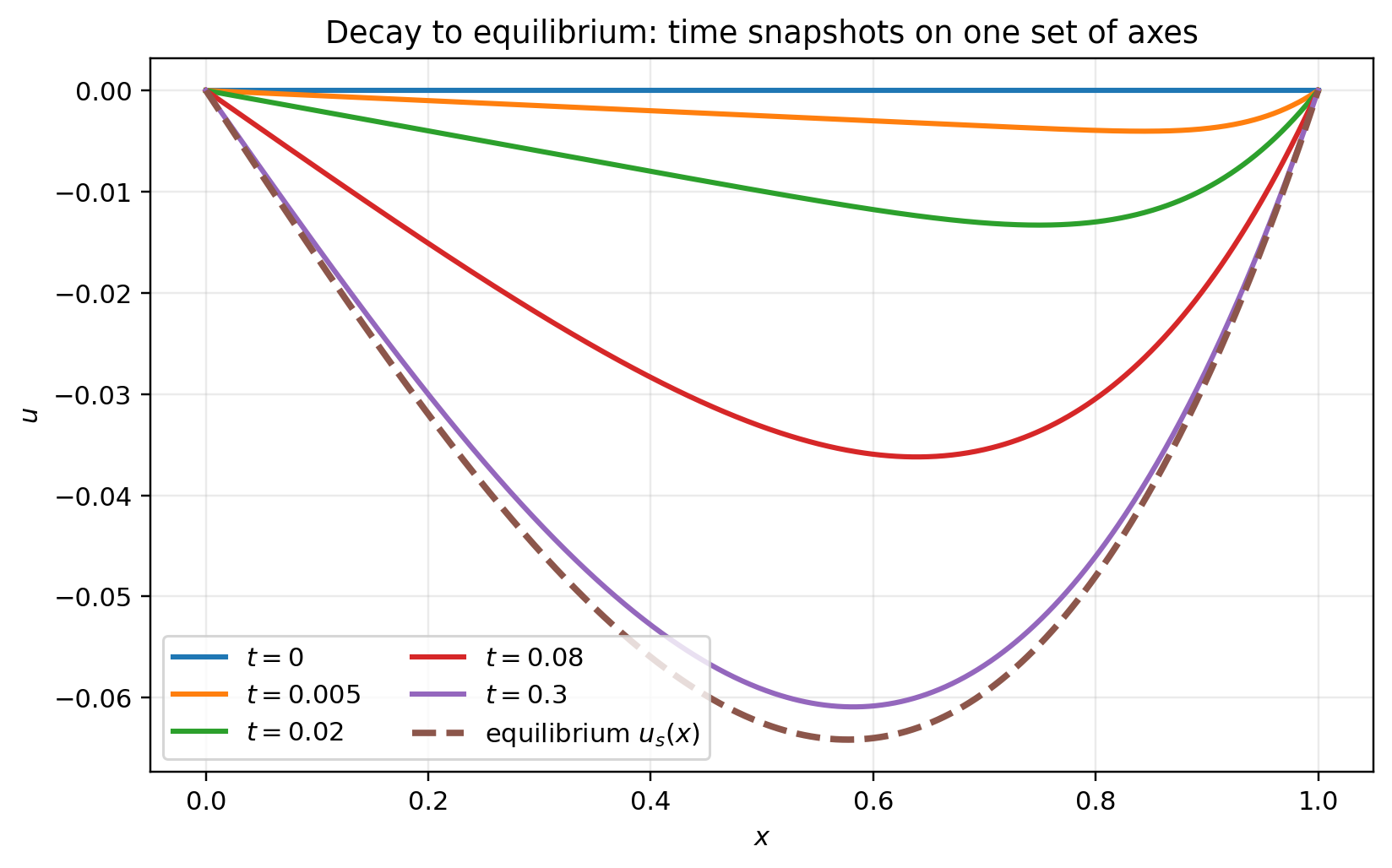
We see the decay of a fully temporal model solution to its equilibrium in Figure 4.2.

For a steady problem \(Lu=f\), the modal coefficients are obtained algebraically when \(\lambda_n\neq0\). If a zero mode is present, its equation instead gives the Fredholm compatibility condition discussed in Chapter 3, and that coefficient is not determined by division by the eigenvalue. For the time-dependent problem \(u_t=Lu+h\), the same spatial eigenbasis gives an ODE for each modal amplitude. This is the basic pattern that persists through the extensions below.

4.5 Extending the model

The prototype \[ u_t=Lu+h \] used a first-order time derivative and a one-dimensional spatial operator. The point of the modal method is that both of these choices can be changed without changing the underlying strategy.

What can we change while keeping the modal strategy?

There are two obvious directions:

change the time operator;
change the spatial problem, for example by moving to several spatial dimensions.

In both cases the spatial eigenfunctions remain the organising basis. What changes is the equation satisfied by each modal amplitude.

We start with the simpler extension.

4.5.1 Changing the time operator

Start with a simple example: \[ \pder{u}{t}{2} = L u + h(x,t). \] This requires an extra initial condition, e.g. \[ u(x,0) = g_1(x),\quad \ddy{u}{t}{\Large\vert}_{t=0} = g_2(x). \] We follow the steps outlined in the initial section:

Assume a series solution: \[ u(x,t) = \sum_n c_n(t)y_n(x),\quad L y_n=-\lambda_n y_n. \]
Substitute into the equation and decompose the forcing: \[ h(x,t) = \sum_n h_n(t)y_n(x). \]
Solve the modal equation; this is the part of the recipe that changes: \[ \deriv{c_n}{t}{2} +\lambda_n c_n - h_n = 0. \]

For \(\lambda_n>0\), the homogeneous part \(c_{nh}\) takes the form: \[ c_{nh}(t) = a_{1n} \sin(\sqrt{\lambda_n}t) + a_{2n}\cos(\sqrt{\lambda_n}t). \] If \(\lambda_n=0\) the homogeneous solution is \(a_{1n}t+a_{2n}\), while \(\lambda_n<0\) gives exponential (equivalently hyperbolic) behaviour.

As we saw in Chapter 2, positive \(\lambda_n\) produces oscillatory wave-like modal behaviour.

More generally we can consider a linear time-dependent operator \(L_t\). For each spatial eigenmode we obtain an equation of the form \[ L_t c_n+\lambda_n c_n=h_n(t). \] If we define the modal time operator \[ M_n=L_t+\lambda_n I, \] then this is simply \[ M_n c_n=h_n(t). \]

This is again an inhomogeneous linear differential equation of the form \[ Ly=f, \] but now the independent variable is time rather than space.

We can do it!! There is, however, one big difference. In the usual time-dependent problem we prescribe all the required data at the initial time, so this is an initial value problem rather than a boundary-value problem. For linear ODE systems with suitably continuous coefficients, the corresponding IVP has a unique solution on the interval on which those coefficients are defined.

Predicting the future… ::: {#fig-nopredict}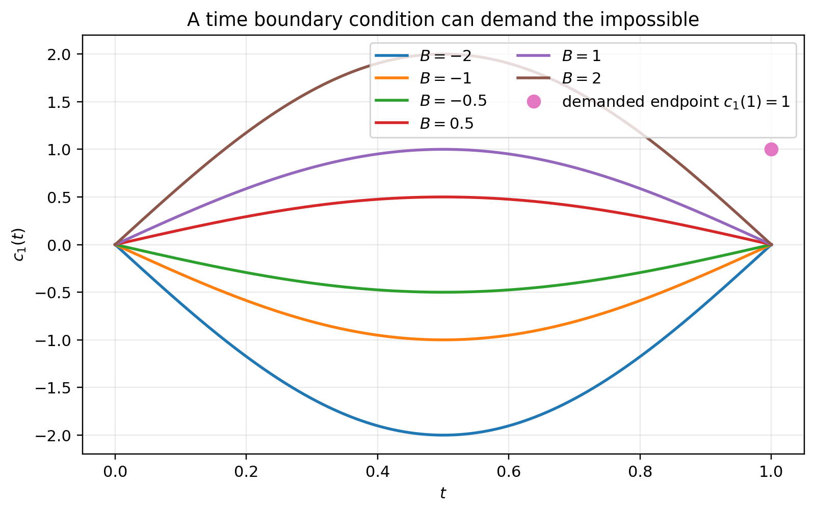

The failure to satisfy the temporal boundary conditions (predicting the future) of a PDE model. :::

If we try to impose a time condition at some \(t_1>0\), it becomes a boundary-value problem in time. For the second-order example above, two conditions suffice and we could impose: \[ u(x,0) = g_0(x),\quad u(x,t_1)=g_1(x). \] That is, we demand, after some time \(t_1\), the function \(u\) takes a very specific spatial profile \(g_1(x)\). Then we cannot guarantee the solution exists, and the same boundary-value/Fredholm machinery may be needed to determine whether the problem can be solved.

An example of this failure is shown in figure ?fig-nopredict which illustrates part of the conclusion to the following problem.

Example: Can we demand what a vibrating string looks like in the future?

Consider the wave equation for a string fixed at both ends:

\[ \frac{\partial^2u}{\partial t^2} = \frac{\partial^2u}{\partial x^2}, \qquad 0<x<1, \]

with

\[ u(0,t)=u(1,t)=0. \]

Suppose the string starts perfectly flat:

\[ u(x,0)=0. \]

Instead of specifying its initial velocity, let’s try something different. We demand that at time \(t=1\) the string has the shape

\[ u(x,1)=\sin(\pi x). \]

Can we find a solution which does that?

Step 1: Separate the spatial modes

The familiar spatial eigenfunctions are

\[ y_n(x)=\sin(n\pi x), \qquad \lambda_n=n^2\pi^2. \]

Expanding the solution,

\[ u(x,t)=\sum_{n=1}^{\infty}c_n(t)\sin(n\pi x), \]

gives a temporal equation for each mode:

\[ \frac{\mathrm{d}^2c_n}{\mathrm{d}t^2} +n^2\pi^2c_n=0. \]

The general solution is

\[ c_n(t)=A_n\cos(n\pi t)+B_n\sin(n\pi t). \]

Because the string starts flat, \(c_n(0)=0\), so \(A_n=0\) for every mode. Thus

\[ u(x,t)= \sum_{n=1}^{\infty} B_n\sin(n\pi t)\sin(n\pi x). \]

Step 2: Look at the future time

At \(t=1\),

\[ \sin(n\pi)=0 \]

for every positive integer \(n\)!

Consequently,

\[ u(x,1)=0 \]

regardless of how we choose the coefficients \(B_n\).

Our demand that

\[ u(x,1)=\sin(\pi x) \]

is impossible.

There is no solution satisfying all the conditions we imposed.

Step 3: What if we demand that the string is flat again?

Now change the future condition to

\[ u(x,1)=0. \]

This time the problem has solutions – rather a lot of them!

For example,

\[ u(x,t)=B\sin(\pi t)\sin(\pi x) \]

works for any constant \(B\).

The string could remain stationary, vibrate gently, or vibrate with a large amplitude. All these possibilities satisfy our conditions at \(t=0\) and \(t=1\).

So the problem is now solvable, but the solution is not unique.

What’s happened?

For the first mode, we were trying to solve the temporal boundary-value problem

\[ c_1''+\pi^2c_1=0, \qquad c_1(0)=0, \qquad c_1(1)=b. \]

But its solutions have the form

\[ c_1(t)=B\sin(\pi t), \]

which means \(c_1(1)=0\) for every \(B\).

If \(b\neq0\), there is no solution. If \(b=0\), there are infinitely many.

This is the same kind of solvability and non-uniqueness issue we encountered with zero eigenvalues in Chapter 3, now appearing in a boundary-value problem in time.

For comparison, if we instead prescribe the initial velocity,

\[ \frac{\partial u}{\partial t}(x,0) = \pi\sin(\pi x), \]

then the initial-value problem determines

\[ u(x,t)=\sin(\pi t)\sin(\pi x). \]

We can predict its future from its initial position and velocity, but we cannot necessarily prescribe an arbitrary future position and expect the equation to accommodate our wishes!

The mathematics of the problems \[ L u(x) = f(x),\quad L_t u(t) =f(t) \] is mathematically very similar. The practical asymmetry comes from the questions we usually ask. In time it is natural to ask how will the system evolve from where it is now?, which gives an initial-value problem. Spatially we usually specify behaviour on the boundary of a finite domain, which gives a boundary-value problem.

Does it always work out.

The answer is no, but this method is effective for a huge class of problems. In particular if L is self adjoint which means Sturm-Liouville operators. I have prepared a non examinable document exploring the technical requirements required for the method to work which you can find in the non examinable material on the ultra page.

4.5.2 Higher-dimensional spatial problems

Chapter 3 showed that the adjoint, self-adjointness, orthogonality and Fredholm ideas extend naturally to operators on a domain \(\mathcal D\subset\mathbb R^m\). For the PDE \[ \ddy{u}{t}=Lu+h(\mathbf x,t), \] we therefore seek an expansion \[ \boxed{ u(\mathbf x,t)=\sum_{\mathbf n}c_{\mathbf n}(t)y_{\mathbf n}(\mathbf x), } \] where \[ Ly_{\mathbf n}=-\lambda_{\mathbf n}y_{\mathbf n} \] with the required spatial boundary conditions.

The recipe is formally the same as in one dimension. The practical difficulty is finding the spatial eigenfunctions. For simple separable geometries this can still be done explicitly.

4.5.3 Box domains: a tractable higher-dimensional example

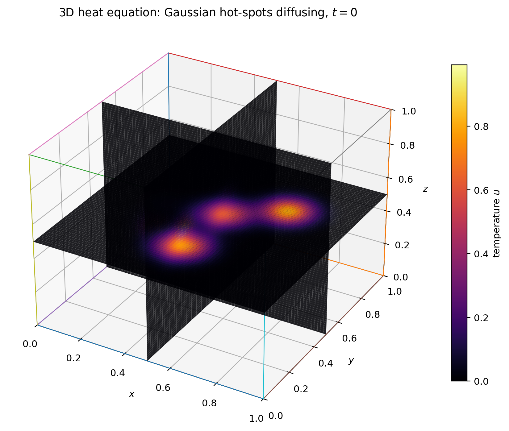
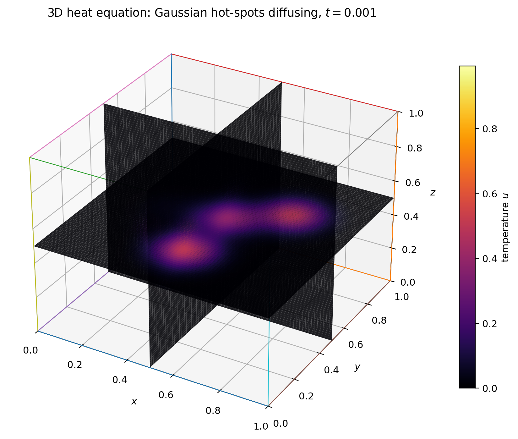
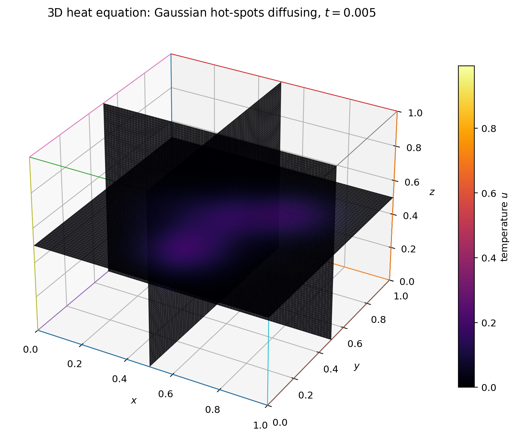
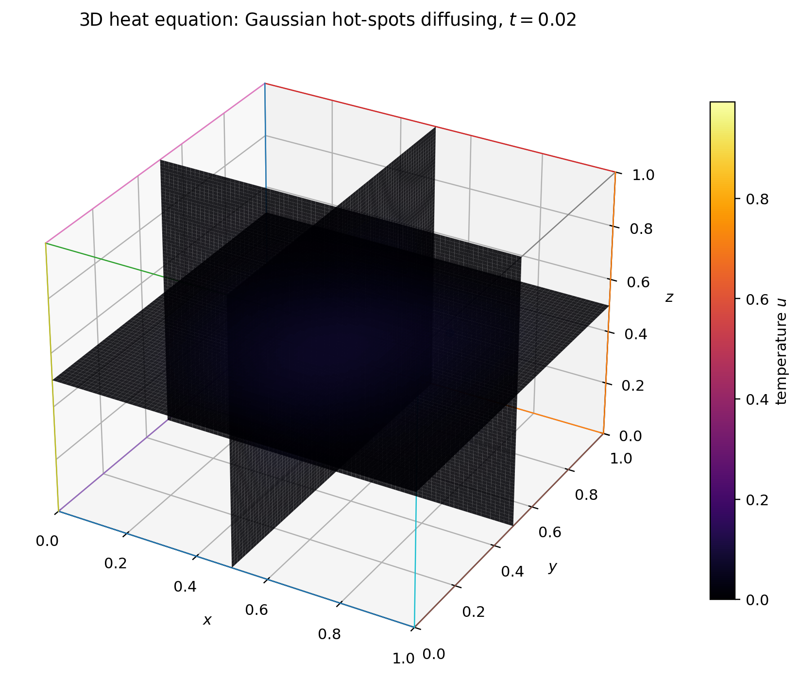
Consider our domain to be a box \([0,L_1]\times[0,L_2]\times\cdots\times[0,L_m]\) with coordinates \((x_1,x_2,x_3, \dots x_m)\).

We consider the Laplacian in Cartesian coordinates: \[ L=\nabla^2=\nabla\cdot\nabla, \qquad \nabla^2u = \sum_{j=1}^m\pder{u}{x_j}{2}. \] We impose Dirichlet boundary conditions: \[\begin{align} & u(0,x_2,x_3\dots x_m)=u(L_1,x_2,x_3\dots x_m) = u(x_1,0,x_3\dots x_m)= u(x_1,L_2,x_3\dots x_m) \\ & \dots=u(x_1,x_2,x_3\dots 0) = u(x_1,x_2,x_3\dots L_m) =0. \end{align}\] We can see the solution to the problem: \[ \nabla^2y_{\mathbf n}=-\lambda_{\mathbf n}y_{\mathbf n} \] is \[ y_{\mathbf n}(\mathbf x) = C_{\mathbf n} \prod_{j=1}^m \sin\left(\frac{n_j\pi x_j}{L_j}\right). \] (we will cover how to derive this in the problem class), with \(n_i=1,2,\ldots\) positive integers, and \[ \lambda_{\mathbf n} = \pi^2 \sum_{j=1}^m\frac{n_j^2}{L_j^2}. \] These eigenfunctions can then be used as the spatial basis for the full PDE expansion, \[ u(\mathbf x,t)=\sum_{n_1=1}^{\infty}\cdots\sum_{n_m=1}^{\infty} c_{n_1,\ldots,n_m}(t) \prod_{j=1}^{m}\sin\left(\frac{n_j\pi x_j}{L_j}\right). \] Each coefficient \(c_{n_1,\ldots,n_m}(t)\) then satisfies the corresponding modal time equation, exactly as in the one-dimensional case.

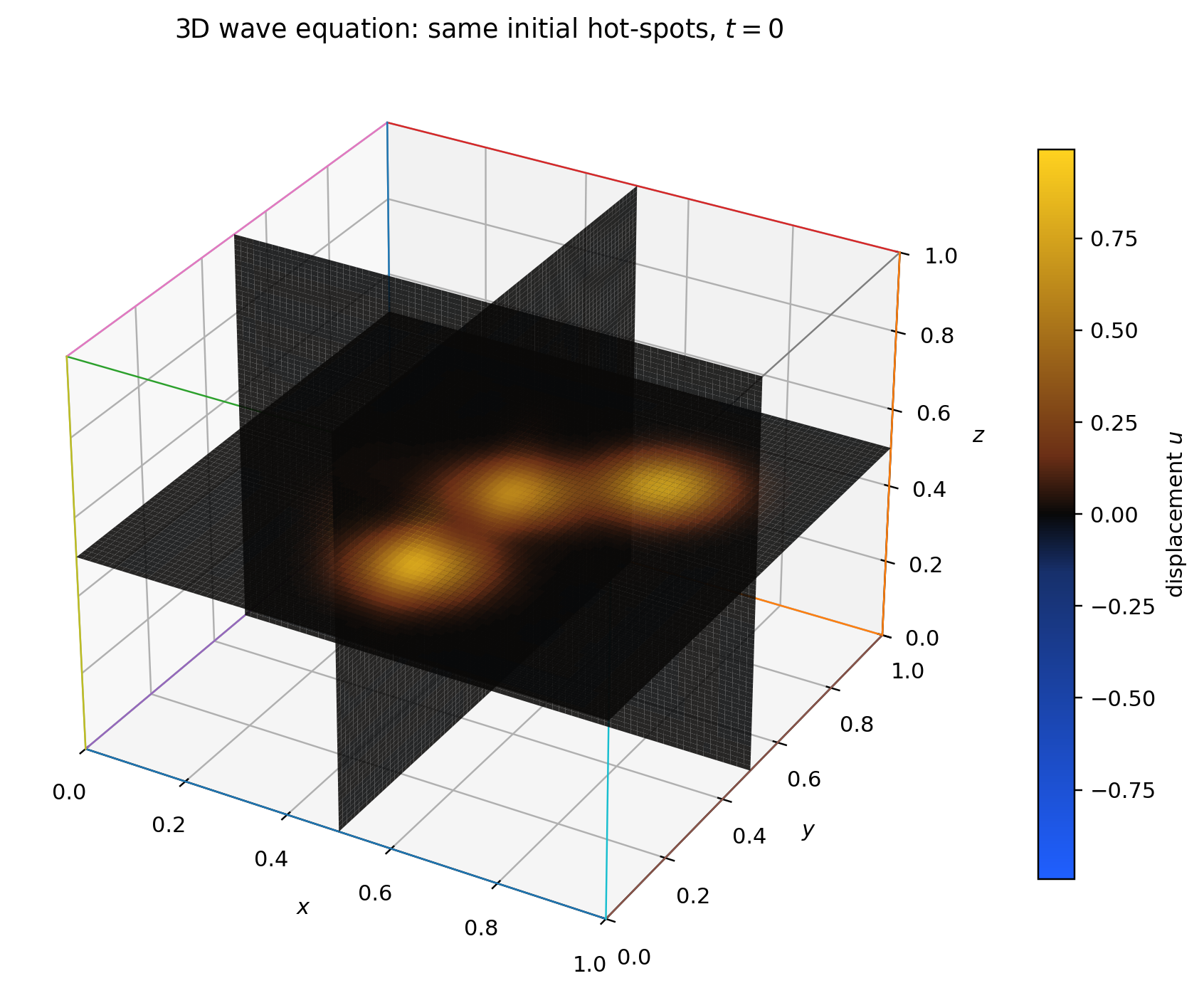
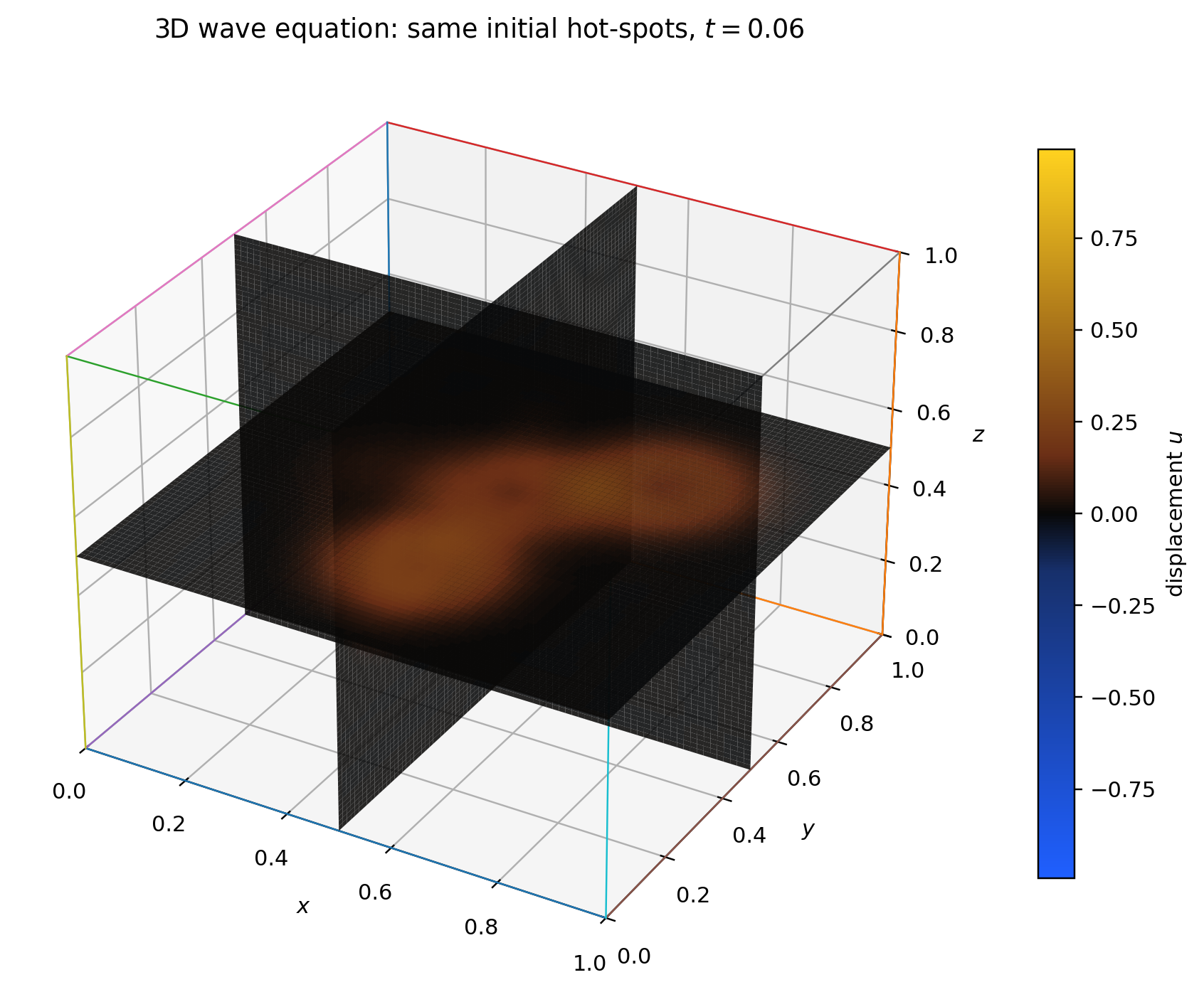
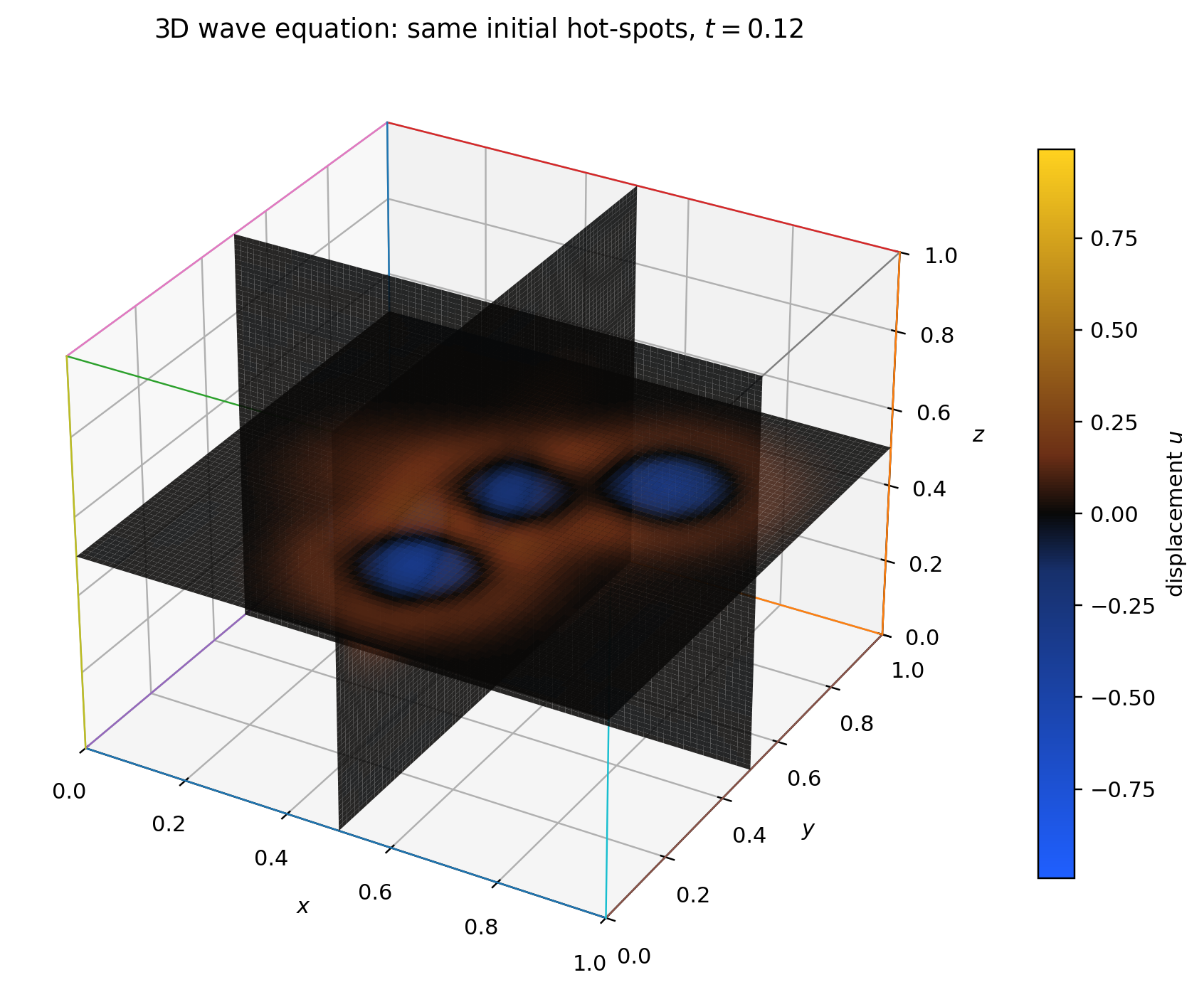
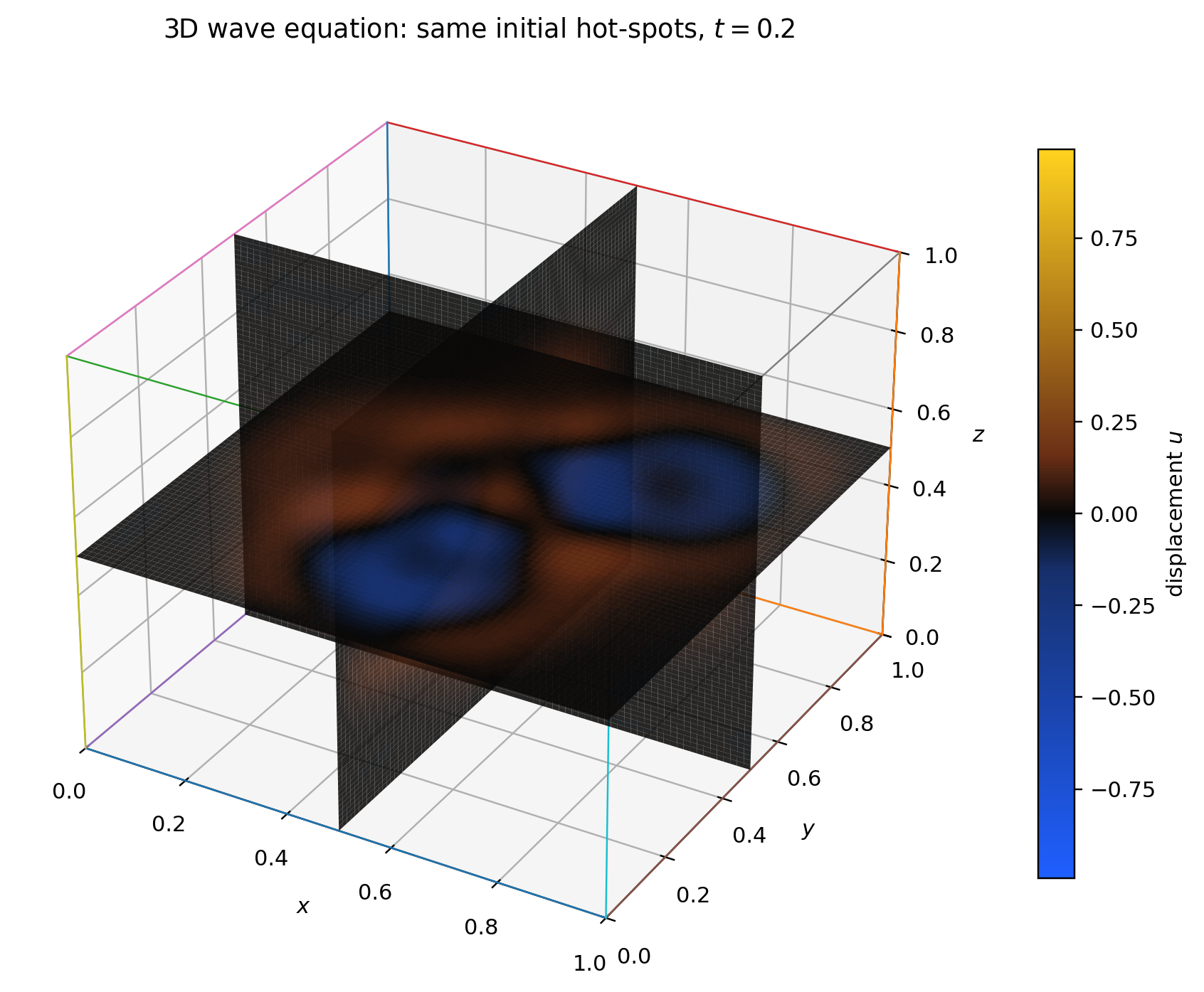
Examples of the 3D heat and wave eqations are shown in Figures Figure 4.4 and ?fig-wave3d.

Example: Heating a circular disc – bringing back the Bessel functions!

Consider the heat equation on a circular disc of radius \(1\):

\[ \frac{\partial u}{\partial t} = \nabla^2u+h(r), \]

where the edge of the disc is held at zero temperature,

\[ u(1,t)=0. \]

Suppose the forcing and initial temperature are both radially symmetric, so there is no dependence on the angular coordinate \(\theta\).

In polar coordinates, our equation becomes

\[ \frac{\partial u}{\partial t} = \frac{1}{r}\frac{\partial}{\partial r} \left(r\frac{\partial u}{\partial r}\right) +h(r). \]

We also require the temperature to remain regular at the centre \(r=0\).

Step 1: Find the spatial eigenfunctions

We met this eigenproblem back in Chapter 2:

\[ \frac{1}{r}\frac{\mathrm{d}}{\mathrm{d}r} \left(r\frac{\mathrm{d}R}{\mathrm{d}r}\right) = -\lambda R. \]

The regular radial eigenfunctions satisfying \(R(1)=0\) are

\[ R_n(r)=J_0(j_{0,n}r), \qquad \lambda_n=j_{0,n}^2, \]

where \(j_{0,n}\) is the \(n\)th positive zero of the Bessel function \(J_0\).

For reference, the first two are approximately

\[ j_{0,1}=2.405, \qquad j_{0,2}=5.520. \]

Step 2: Choose an initial temperature and a forcing

Let’s make the example manageable by choosing

\[ u(r,0)=J_0(j_{0,2}r) \]

and

\[ h(r)=J_0(j_{0,1}r). \]

So the disc initially has the shape of the second radial mode, but we continuously force it with the first radial mode.

We can expand the solution as

\[ u(r,t)= \sum_{n=1}^{\infty}c_n(t)J_0(j_{0,n}r). \]

How do we find the coefficients of the forcing and initial condition?

Remember that the radial Bessel modes are orthogonal with weight \(r\):

\[ \int_0^1 rJ_0(j_{0,m}r)J_0(j_{0,n}r)\,\mathrm{d}r=0, \qquad m\neq n. \]

The weighted coefficient formula therefore tells us that the forcing has just one non-zero coefficient:

\[ h_1=1, \qquad h_n=0\quad(n\neq1). \]

Similarly, the initial condition gives

\[ c_2(0)=1, \qquad c_n(0)=0\quad(n\neq2). \]

Step 3: Solve the temporal equations

Each mode satisfies

\[ \frac{\mathrm{d}c_n}{\mathrm{d}t} +j_{0,n}^2c_n=h_n. \]

For the first mode,

\[ \frac{\mathrm{d}c_1}{\mathrm{d}t} +j_{0,1}^2c_1=1, \qquad c_1(0)=0. \]

Using our temporal solution formula gives

\[ c_1(t)= \frac{1-\mathrm{e}^{-j_{0,1}^2t}}{j_{0,1}^2}. \]

For the second mode there is no forcing, so

\[ \frac{\mathrm{d}c_2}{\mathrm{d}t} +j_{0,2}^2c_2=0, \qquad c_2(0)=1, \]

giving

\[ c_2(t)=\mathrm{e}^{-j_{0,2}^2t}. \]

All the other coefficients remain zero.

Our complete solution is therefore

\[ \begin{aligned} u(r,t) ={}& \frac{1-\mathrm{e}^{-j_{0,1}^2t}}{j_{0,1}^2} J_0(j_{0,1}r)\\ &+ \mathrm{e}^{-j_{0,2}^2t} J_0(j_{0,2}r). \end{aligned} \]

Step 4: What happens to the disc?

The original second radial mode decays away:

\[ \mathrm{e}^{-j_{0,2}^2t}\longrightarrow0. \]

Meanwhile, the forcing builds up the first radial mode until the temperature approaches

\[ u_s(r)=\frac{J_0(j_{0,1}r)}{j_{0,1}^2}. \]

We can check this directly using the steady-state equation

\[ \nabla^2u_s+h=0. \]

Since

\[ \nabla^2J_0(j_{0,1}r) = -j_{0,1}^2J_0(j_{0,1}r), \]

our limiting temperature does indeed solve the steady-state problem.

What was different from the one-dimensional problem?

Surprisingly little!

The spatial modes are now Bessel functions rather than sines or cosines, and we must use the radial weight \(r\) when calculating coefficients. But once we have the eigenfunctions and eigenvalues, the temporal equations are exactly the same as before.

The disc has changed the spatial mathematics, not the overall solution strategy.

4.6 Where the analytic method reaches its limits

The box above is tractable because both the geometry and the operator are separable. The same is true of several important examples we met earlier, including the disc and sphere.

For more complicated geometries, however, the spatial eigenproblem may no longer separate into simple one-dimensional pieces. The eigenfunction method still makes conceptual sense, but finding the eigenfunctions analytically can become the difficult part.

Does it always work out 2

Similar to the 1-D case, I have prepared a non-examinable document exploring the technical requirements required for the method to work in higher dimensions which you can find in the non examinable material on the ultra page.

The rough message is:

\[ \boxed{ \text{simple geometry + suitable operator} \;\Longrightarrow\; \text{explicit spatial modes are often available}, } \]

whereas more complicated geometries generally require other analytic or numerical tools.

This is one of the motivations for Green’s methods, which we consider later in the course.

Before moving on, it is useful to add one final non-examinable perspective: what survives when the PDE itself is nonlinear?

4.7 Beyond linear PDEs: why the modal viewpoint still matters

This final section is non-examinable. Its purpose is to show that the ideas developed in this course remain useful well beyond problems that can be solved analytically.

The eagle-eyed student will note that:

We have largely discussed linear methodologies, and in particular the principle of superposition.
Yet many of the most interesting and realistic examples in physics, chemistry, and biology are non-linear.

So does any of this apply to non-linear PDEs, which generally model real systems more faithfully?

Most nonlinear PDEs must be treated numerically, since analytic solutions are rarely available. A common approach is still to expand the solution in spatial modes. The crucial change is that the nonlinear terms couple those modes together.

4.7.1 Why linear eigen-decompositions still matter

Even though non-linear equations violate superposition, eigen-decomposition remains useful for several reasons:

Efficient representation of structure:
The eigenfunctions of a linear operator (such as the Laplacian) often reflect the geometry and boundary conditions of the problem.
For sufficiently smooth or coherent solutions, expanding in a natural basis often concentrates much of the important physical behaviour in relatively few modes, making the numerical system more compact and efficient.
Mode coupling insight:
In a non-linear PDE, such as the Navier–Stokes or reaction–diffusion equations, non-linearity introduces coupling between modes — energy or information is transferred between eigenmodes.
Expressing the solution in an eigenbasis makes these couplings explicit, helping to analyse phenomena like turbulence, pattern formation, or instability growth.
Stability and time integration:
The linear part of a PDE often dominates its stability properties.
After projection or spatial discretisation, the linear part can often be treated exactly or very accurately in time, while the remaining non-linear terms are handled separately. This is closely related to ideas used in operator splitting and exponential integrators.
Error control and convergence:
Orthogonal spectral bases make it natural to study how much information is retained as the expansion is truncated after \(N\) modes. For sufficiently smooth problems, spectral approximations can converge extremely rapidly.
Analytic and diagnostic value:
Even when not used for computation, decomposing numerical or experimental solutions into eigenmodes helps to interpret results — identifying dominant spatial scales, symmetry breaking, or coherent structures.

Example: When Fourier modes start talking to each other!

Here is a little reward for anyone who has made it this far!

Consider the viscous Burgers equation,

\[ \frac{\partial u}{\partial t} + u\frac{\partial u}{\partial x} = \nu\frac{\partial^2u}{\partial x^2}, \]

on the periodic domain \(0\leq x\leq2\pi\), where \(\nu>0\) is a viscosity coefficient.

The right-hand side describes diffusion, which tends to smooth out the function. The nonlinear term

\[ u\frac{\partial u}{\partial x} \]

describes transport by a velocity which depends on the solution itself.

This is a simplified cousin of the nonlinear advection appearing in the Navier–Stokes equations.

Let’s start with just one mode

Suppose our initial condition is

\[ u(x,0)=A\sin x. \]

If we had only the diffusion term, we could immediately write

\[ u(x,t)=A\mathrm{e}^{-\nu t}\sin x. \]

The sine mode would simply decay. No other modes would appear.

But what happens when we include the nonlinear term?

At \(t=0\),

\[ u=A\sin x, \qquad \frac{\partial u}{\partial x}=A\cos x. \]

Therefore

\[ u\frac{\partial u}{\partial x} = A^2\sin x\cos x. \]

Using the trigonometric identity

\[ \sin x\cos x=\frac12\sin(2x), \]

we obtain

\[ u\frac{\partial u}{\partial x} = \frac{A^2}{2}\sin(2x). \]

Look what has happened!

We started with \(\sin x\), but the nonlinear term has produced \(\sin(2x)\).

The PDE tells us that the initial rate of change is

\[ \left.\frac{\partial u}{\partial t}\right|_{t=0} = -\nu A\sin x -\frac{A^2}{2}\sin(2x). \]

So, for a sufficiently short time \(\Delta t\),

\[ \begin{aligned} u(x,\Delta t)\approx{}& A(1-\nu\Delta t)\sin x\\ &-\frac{A^2\Delta t}{2}\sin(2x). \end{aligned} \]

The second Fourier mode has appeared, even though it was completely absent from the initial condition.

And it doesn’t stop there!

Once the solution contains both \(\sin x\) and \(\sin(2x)\), the nonlinear term multiplies these functions together. Their products contain \(\sin(3x)\), and interactions involving the new modes can generate still higher harmonics.

The modes are no longer independent.

For example, if we approximate the solution using only two modes,

\[ u(x,t)\approx a(t)\sin x+b(t)\sin(2x), \]

and project Burgers’ equation onto those two Fourier modes, we obtain

\[ \frac{\mathrm{d}a}{\mathrm{d}t} = -\nu a+\frac12 ab, \]

\[ \frac{\mathrm{d}b}{\mathrm{d}t} = -4\nu b-\frac12 a^2. \]

Compare these with the independent modal equations we derived for linear PDEs!

The rate of change of \(a\) now depends on \(b\), and the rate of change of \(b\) depends on \(a\). The nonlinear terms have coupled the modes.

This two-mode system is an approximation: the full nonlinear PDE also generates modes we have left out. Including more modes gives a larger system of coupled ODEs.

So was everything we learned about eigenfunction expansions wasted?

Quite the opposite!

We have still reduced a PDE to equations for modal amplitudes, just as we did throughout this chapter. The difference is that we must now solve those equations together, rather than one at a time.

The Fourier basis has not stopped being useful. It has given us a way to see exactly how the nonlinearity transfers information between different spatial scales.

This is one of the central ideas behind spectral methods for nonlinear PDEs, including models of fluid flow and turbulence.

4.8 Summary

The central model in this chapter was

\[ \boxed{ u_t=Lu+h(\mathbf x,t), } \]

together with boundary and initial conditions.

Using the theory developed in Chapters 1–3, we saw that the solution strategy is:

solve the spatial eigenvalue problem for \(L\) with the required boundary conditions;
expand the solution, forcing and initial data in those spatial modes;
use \[ Ly_n=-\lambda_n y_n \] to turn the spatial differential operator into multiplication by an eigenvalue;
solve the resulting equations for the modal amplitudes.

Thus

\[ \boxed{ \text{spatial eigenproblem} \;\longrightarrow\; \text{mode expansion} \;\longrightarrow\; \text{equations for modal amplitudes}. } \]

We then saw that the same philosophy survives several extensions:

steady states reduce to the Chapter 3 problem \[ Lu=f; \]
changing the time operator changes the modal time equation, but not the spatial basis;
moving to higher dimensions changes the spatial eigenproblem, but not the overall method;
in nonlinear problems the modes generally become coupled, but the modal viewpoint remains useful analytically and numerically.

The broad lesson is therefore

\[ \boxed{ \text{the spatial eigenproblem determines the modes;} \qquad \text{the rest of the PDE determines what those modes do.} } \]

For simple geometries the spatial modes can often be found analytically. For more complicated geometries or operators, finding the spatial response becomes the difficult step and motivates other methods, including Green’s methods.

4.1 A general linear PDE model

4.1.1 The operator

4.1.2 The “source/forcing” term \(h(x,t)\)

4.1.3 Boundary conditions

4.1.4 Initial conditions

4.1.5 Where does this model occur?

4.1.6 Some applied examples

4.2 Solving the model by eigenfunction expansion

4.3 A concrete forced Fourier example

4.4 Steady states: recovering \(Lu=f\)

4.5 Extending the model

4.5.1 Changing the time operator

4.5.2 Higher-dimensional spatial problems

4.5.3 Box domains: a tractable higher-dimensional example

4.6 Where the analytic method reaches its limits

4.7 Beyond linear PDEs: why the modal viewpoint still matters

4.7.1 Why linear eigen-decompositions still matter

4.7.2 Spectral and modal methods in practice

4.8 Summary