$$ \def\ab{\boldsymbol{a}} \def\bb{\boldsymbol{b}} \def\cb{\boldsymbol{c}} \def\db{\boldsymbol{d}} \def\eb{\boldsymbol{e}} \def\fb{\boldsymbol{f}} \def\gb{\boldsymbol{g}} \def\hb{\boldsymbol{h}} \def\kb{\boldsymbol{k}} \def\nb{\boldsymbol{n}} \def\tb{\boldsymbol{t}} \def\ub{\boldsymbol{u}} \def\vb{\boldsymbol{v}} \def\xb{\boldsymbol{x}} \def\yb{\boldsymbol{y}} \def\Ab{\boldsymbol{A}} \def\Bb{\boldsymbol{B}} \def\Cb{\boldsymbol{C}} \def\Eb{\boldsymbol{E}} \def\Fb{\boldsymbol{F}} \def\Jb{\boldsymbol{J}} \def\Lb{\boldsymbol{L}} \def\Rb{\boldsymbol{R}} \def\Ub{\boldsymbol{U}} \def\xib{\boldsymbol{\xi}} \def\evx{\boldsymbol{e}_x} \def\evy{\boldsymbol{e}_y} \def\evz{\boldsymbol{e}_z} \def\evr{\boldsymbol{e}_r} \def\evt{\boldsymbol{e}_\theta} \def\evp{\boldsymbol{e}_r} \def\evf{\boldsymbol{e}_\phi} \def\evb{\boldsymbol{e}_\parallel} \def\omb{\boldsymbol{\omega}} \def\dA{\;d\Ab} \def\dS{\;d\boldsymbol{S}} \def\dV{\;dV} \def\dl{\mathrm{d}\boldsymbol{l}} \def\rmd{\mathrm{d}} \def\bfzero{\boldsymbol{0}} \def\Rey{\mathrm{Re}} \def\Real{\mathbb{R}} \def\grad{\boldsymbol\nabla} \newcommand{\dds}[2]{\frac{d{#1}}{d{#2}}} \newcommand{\ddy}[2]{\frac{\partial{#1}}{\partial{#2}}} \newcommand{\pder}[3]{\frac{\partial^{#3}{#1}}{\partial{#2}^{#3}}} \newcommand{\deriv}[3]{\frac{d^{#3}{#1}}{d{#2}^{#3}}} \newcommand{\ddt}[1]{\frac{d{#1}}{dt}} \newcommand{\DDt}[1]{\frac{\mathrm{D}{#1}}{\mathrm{D}t}} \newcommand{\been}{\begin{enumerate}} \newcommand{\enen}{\end{enumerate}}\newcommand{\beit}{\begin{itemize}} \newcommand{\enit}{\end{itemize}} \newcommand{\nibf}[1]{\noindent{\bf#1}} \renewcommand{\vec}{\mathbfit} \def\bra{\langle} \def\ket{\rangle} \renewcommand{\S}{{\cal S}} \newcommand{\wo}{w_0} \newcommand{\wid}{\hat{w}} \newcommand{\taus}{\tau_*} \newcommand{\woc}{\wo^{(c)}} \newcommand{\dl}{\mbox{$\Delta L$}} \newcommand{\upd}{\mathrm{d}} \newcommand{\dL}{\mbox{$\Delta L$}} \newcommand{\rs}{\rho_s} $$
Throughout this chapter, keep the following question in mind:
Can we understand a complicated object by decomposing it into simple, independent pieces?
This idea will reappear repeatedly throughout the rest of the course.
1.1 A recap of the Fourier series
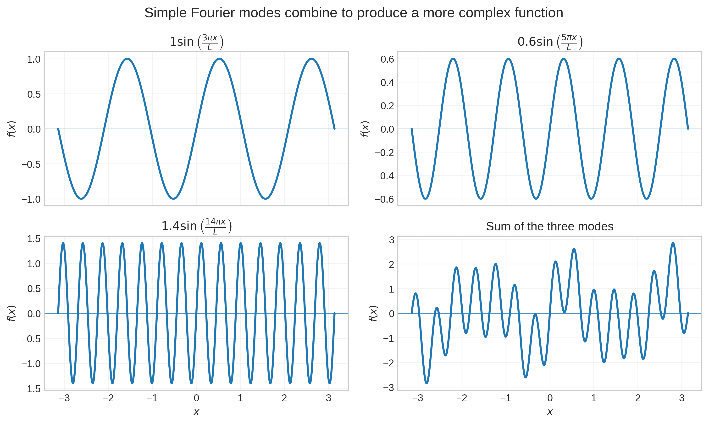
In Calculus I you were introduced to the Fourier series. The crucial idea is we can represent any suitably smooth function \(f(x)\) defined on \([-L,L]\) as a Fourier series \[ f(x)=a_0 +\sum_{n=1}^{\infty}\left[ a_n\cos\!\Big(\frac{n\pi x}{L}\Big) +b_n\sin\!\Big(\frac{n\pi x}{L}\Big) \right]. \]
To make this recreate a specific function we have to calculate the coefficients using the following formulae: \[\begin{align} &a_0=\frac{1}{2L}\int_{-L}^L f(x)\,\mathrm{d}x,\,\quad a_n=\frac{1}{L}\int_{-L}^L f(x)\cos\!\Big(\frac{n\pi x}{L}\Big)\,\mathrm{d}x,\,\\ &b_n=\frac{1}{L}\int_{-L}^L f(x)\sin\!\Big(\frac{n\pi x}{L}\Big)\,\mathrm{d}x. \end{align}\]
The basic idea is illustrated in Figure 1.1. We see three examples of specific components (values of \(n\)) which are simple sine/cosines, then in the fourth panel we see combining them leads to a more complex function. In short we construct complexity from simplicity
We will use the word mode throughout these notes for one of the simple components in such a decomposition.
For a Fourier series,
\[ 1,\qquad \cos\left(\frac{n\pi x}{L}\right), \qquad \sin\left(\frac{n\pi x}{L}\right) \]
are the Fourier modes, and the coefficients \(a_n,b_n\) tell us how much of each mode is present in the function.
More generally, if
\[ f(x)=\sum_n c_n\psi_n(x), \]
we will often refer to the basis functions \(\psi_n\) as the modes of the decomposition. Later, when solving PDEs, the natural modes will be selected by a differential operator together with its boundary conditions.
So a mode decomposition simply means representing a complicated object as a sum of simpler components whose amplitudes can be studied separately.
To illustrate the power of this idea let’s look at some examples. We consider a partial Fourier series \(f_N\) of order \(N\):
\[ f_N(x)=a_0 +\sum_{n=1}^{N}\left[ a_n\cos\!\Big(\frac{n\pi x}{L}\Big) +b_n\sin\!\Big(\frac{n\pi x}{L}\Big) \right]. \]
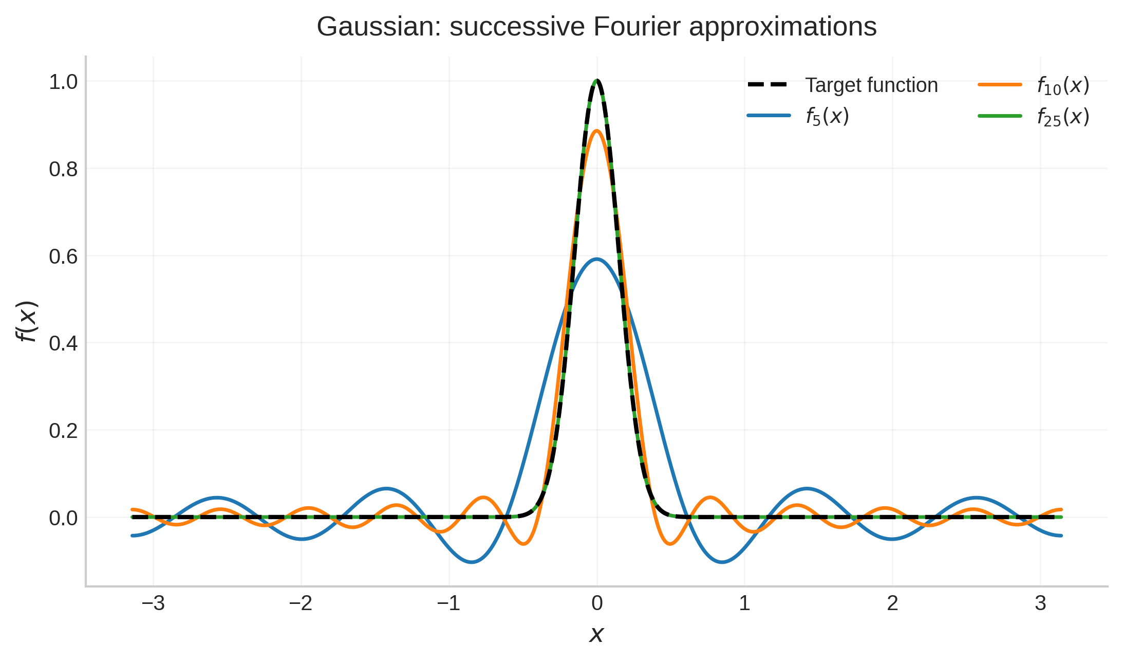
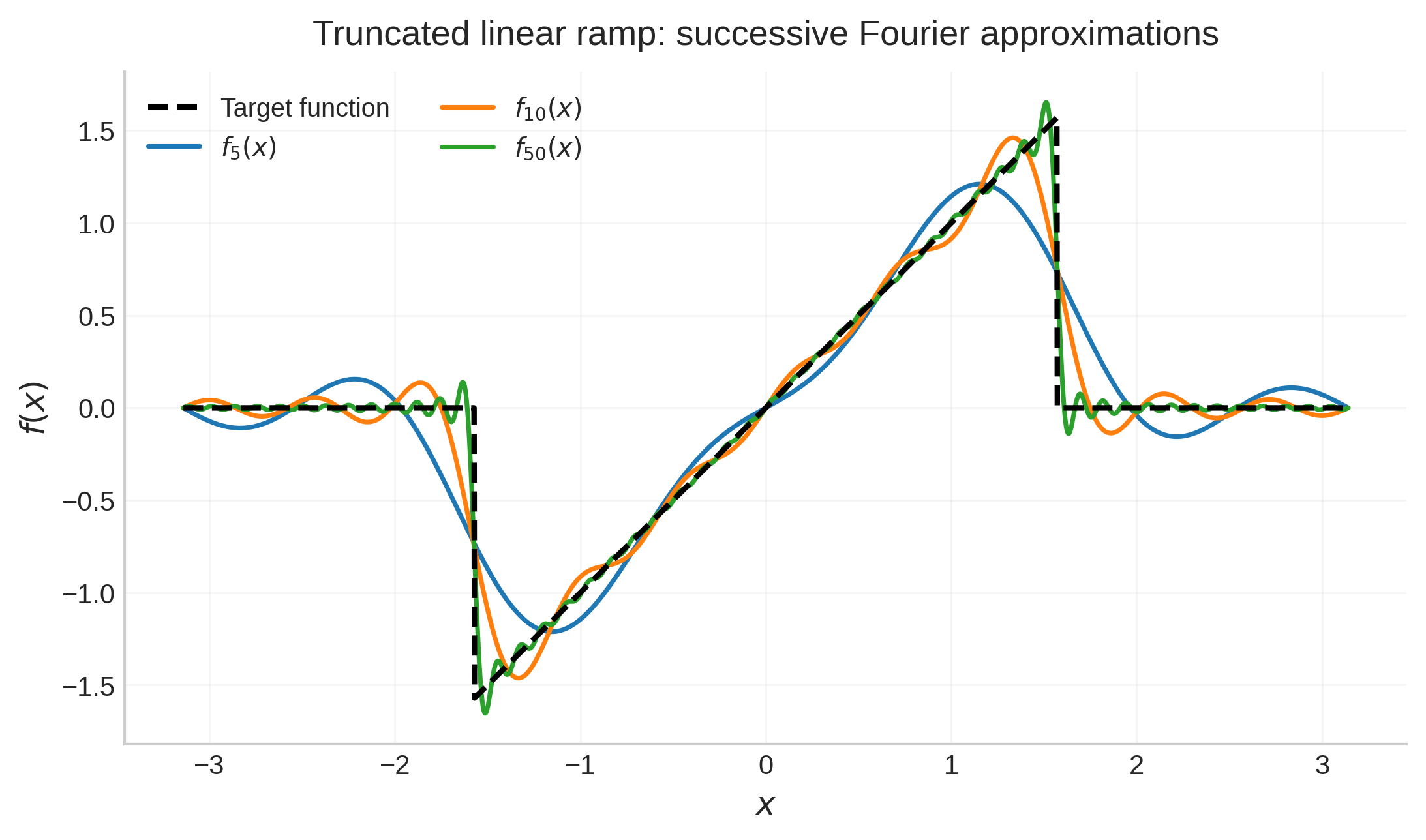
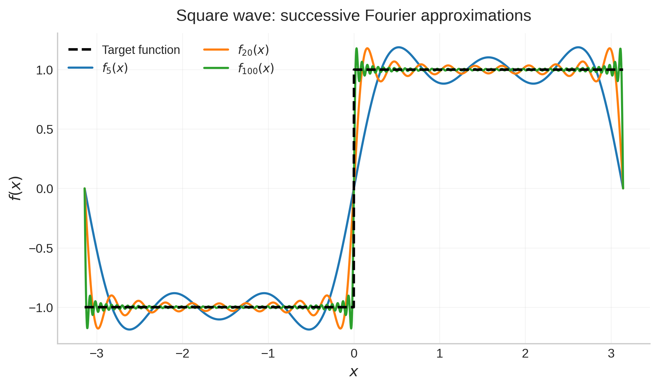
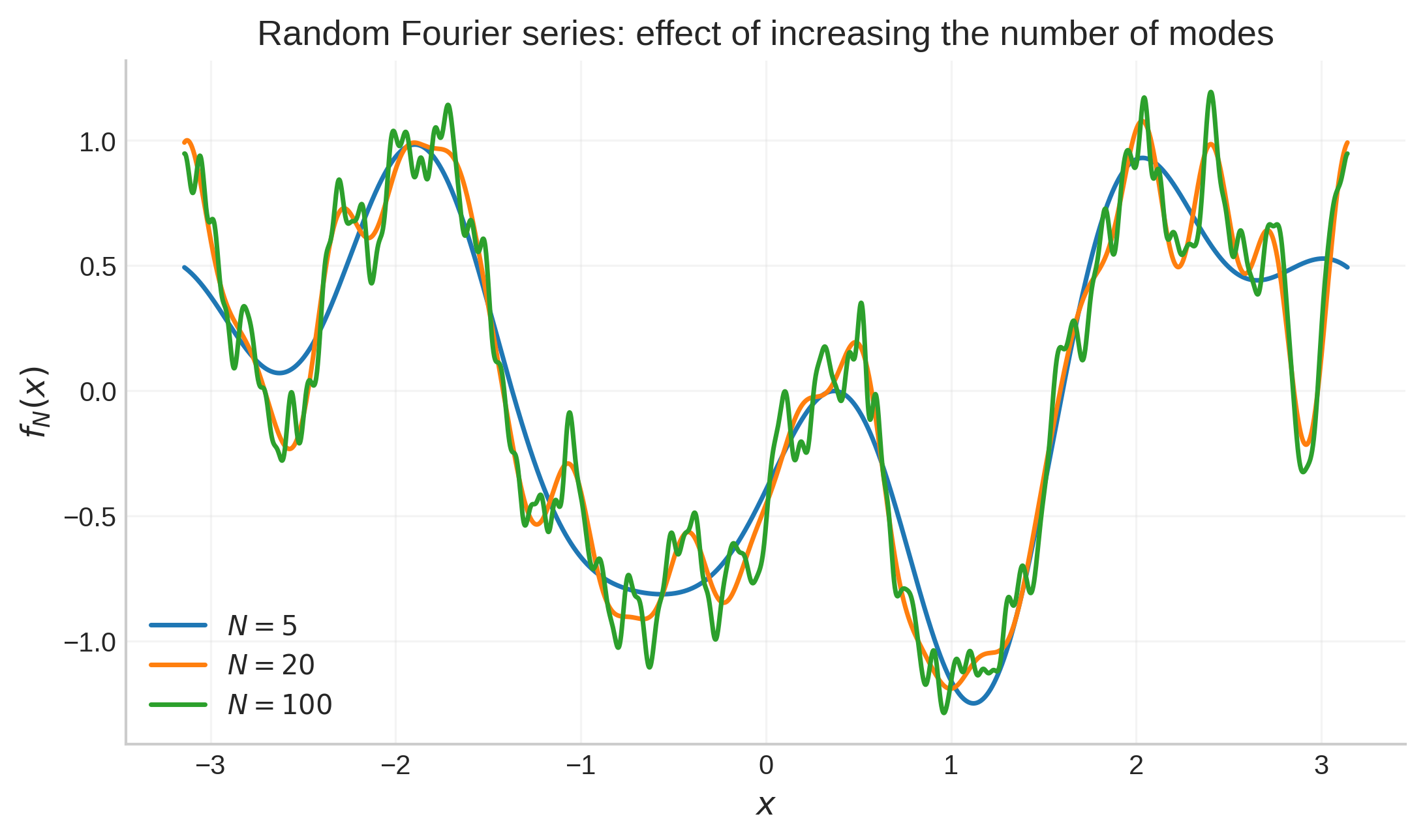
In Figure 1.2 we see a number of examples of this function plotted as \(N\) is increased, and compared to the function \(f(x)\) itself. The partial sum \(f_N(x)\) gets closer to the function \(f(x)\) as \(N\) increases. Indeed, as \(N\rightarrow\infty\), the Fourier series converges to \(f(x)\) at points where the periodic extension is continuous, and to the midpoint of the two limiting values at a jump. More generally, the series converges to \(f\) in the \(L^2\) sense, a notion we will introduce shortly. We will return to this convergence later.
Question 1 of the week 6 problem sheet will walk you through the notion of convergence in the \(L^2\) norm.
Questions 5 concerns truncation and accuracy.
Note that some of these functions are not differentiable or even continous, yet sine and cosine are infinitely differentiable….
I will show you how to use this colab notebook in class to calculate and plot your own Fourier series. I would encourage you to try it out and get a feel for how accurate the series is if you don’t sum all the way to infinity. This finite sum limitation (truncation) is a crucial practical issue (not examinable in this course)!
We now focus on some aspects of the Fourier series which we will find are very much generalisable.
1.1.1 Finite vs infinite dimensional vector spaces
An analogy which is crucial to linking much of what we will discuss in this half of your course to linear algebra is the structural similarity of vectors/matrices and the Fourier series:
Basis representations and components
You have seen that an arbitrary vector \(\vec{a}\in \mathbb{R}^n\) can be represented in terms of some basis \(\left\{\vec{e}_i\right\}_{i=1}^{n}\), let’s make \(n=3\) to be concrete:
\[ \vec{a} = a_1 \vec{e}_1 + a_2 \vec{e}_2 + a_3 \vec{e}_3. \]
The simple idea is we can represent the object, the vector, as a set of real numbers \((a_1,a_2,a_3)\), then, as you saw in the first half of this course you can represent three-dimensional curves \(\vec{c}(t)\) via real-valued functions: \[ \vec{c}(t) = a_1(t)\vec{e}_1 + a_2(t)\vec{e}_2 + a_3(t)\vec{e}_3 \] and surfaces \(\vec{S}(u,v)\): \[ \vec{S}(u,v) = a_1(u,v)\vec{e}_1 + a_2(u,v)\vec{e}_2 + a_3(u,v)\vec{e}_3. \]
The idea with the Fourier series is that there is a basis \(\left\{1\right\}\cup\left\{\cos(n \theta),\sin(n\theta)\right\}_{n=1}^{\infty}\) and the function is specified by the set of coefficients \(\left\{a_n,b_n\right\}_{n=1}^{\infty}\) together with the constant coefficient \(a_0\).
This is an example of an infinite dimensional vector space; you saw some in linear algebra last year (Chapter 2 Epiphany). As we will see a lot of the properties are identical to the finite dimensional case, but we have to add on the complication that we need these series to converge which was largely ignored last year.
Similar to the vector case we can make these coefficients depend on another parameter, which could be time \(t\):
\[ f(x,t)=a_0 +\sum_{n=1}^{\infty}\left[ a_n(t)\cos\!\Big(\frac{n\pi x}{L}\Big) +b_n(t)\sin\!\Big(\frac{n\pi x}{L}\Big) \right]. \]
This is a bit like an infinite dimensional curve! We will see such objects when we start studying partial differential equations in chapter 2. A simple example you have seen already in term 2 of Calculus I is the solution to the heat equation for a function \(f(x,t)\in[0,L]\times(0,\infty)\): \[ \ddy{f}{t} = D\pder{f}{x}{2}, \tag{1.1}\]
which, if we assume the function \(f(x,t)\) is zero on the boundaries of its spatial domain \(x\in[0,L]\), is:
\[ f(x,t) = \sum_{n=1}^{\infty}a_n\mathrm{e}^{-D\frac{n^2}{L^2}\pi^2 t}\sin\left(\frac{n\pi x}{L}\right). \tag{1.2}\] for some constants \(a_n\) (specified by stating the value of \(f(x,0)\) as a Fourier series).
Confirm by partial differentiation that inserting Equation 1.2 into Equation 1.1 leads to the equation being satisfied, and further that it satisfies the stated boundary conditions \(f(0,t)=f(L,t)=0\).
In the video above we see an example of the solution Equation 1.2 in which, as time increases, each of the coefficients decays exponentially. The higher \(n\) (the higher the frequency of the sinusoid) the faster it decays. Thus the function first simplifies by losing its fine scales (smooths out) before eventually the lower frequency component \(n=1\) is left decaying slowly to zero.
Why does \(a_0=0\) for this solution?
Orthogonality and the coefficient grab. With vectors we can, for a given \(\vec{a}\), find its \(k^{\text{th}}\) component using the coefficient grab method: \[ \vec{a}\cdot{\vec{e_k}} = (a_1 \vec{e}_1 + a_2 \vec{e}_2 + \dots a_n\vec{e}_n)\cdot\vec{e_k} = a_k\vec{e}_k\cdot\vec{e}_k, \] where we have used orthogonality, \(\vec{e}_i\cdot\vec{e}_j = 0\) unless \(i=j\), for the last step. Then we have the coefficient formula: \[ a_k = \frac{\vec{a}\cdot{\vec{e_k}}}{\vec{e}_k\cdot\vec{e}_k}. \] This formula is used to obtain the set \(\left\{a_k \right\}_{k=1}^{n}\).
To my knowledge I am the only person who calls it this (the coefficient grab), but it’s my course and it makes sense to me as its descriptive of what the aim of the operation is, so……..
For those who like to be formally correct; \(a_k\) is the projection of the vector \(\vec{a}\) onto the basis component \(\vec{e}_k\).
Usually we would choose a basis to be orthonormal \(\vec{e}_i\cdot\vec{e}_j = \delta_{ij}\) so we don’t need the denominator.
Before writing the Fourier modes on a general interval \([a,b]\), note that its length is \(b-a\). The equivalent full Fourier modes therefore have frequency \(2n\pi/(b-a)\); setting \(b-a=2L\) recovers the \(n\pi/L\) form used above.
The exact same coefficient grab procedure is used for the infinite dimensional Fourier series. This relies on the following orthogonalities on a domain \([a,b]\):
For integers \(m \neq n\), \[ \int_a^b \cos\!\left(\frac{2n\pi(x-a)}{b-a}\right) \cos\!\left(\frac{2m\pi(x-a)}{b-a}\right)\,\mathrm{d}x = 0, \] and likewise for the sine terms.
Also, \[ \int_a^b \cos\!\left(\frac{2n\pi(x-a)}{b-a}\right) \sin\!\left(\frac{2m\pi(x-a)}{b-a}\right)\,\mathrm{d}x =0, \] for any \(n,m\).
You proved these results in Calculus 1 last year. It would be good practice for you to re-derive them.
These orthogonality conditions give us the a coefficient grab method, which works exactly as in the vector case. Say we want the \(m^{\text{th}}\) \(\cos\) coefficient of the series (\(a_m\)): \[ f(x)=a_0 +\sum_{n=1}^{\infty}\left[ a_n\cos\!\left(\frac{2n\pi(x-a)}{b-a}\right) +b_n\sin\!\left(\frac{2n\pi(x-a)}{b-a}\right) \right]. \] We multiply by \(\cos\) and integrate to enforce the orthogonality: \[\begin{align} &\int_a^b f(x)\cos\!\left(\frac{2m\pi(x-a)}{b-a}\right)\,\mathrm{d}x =\int_a^b\cos\!\left(\frac{2m\pi(x-a)}{b-a}\right) \left\{a_0+\sum_{n=1}^{\infty}\left[ a_n\cos\!\Big(\frac{2n\pi (x-a)}{b-a}\Big) +b_n\sin\!\Big(\frac{2n\pi (x-a)}{b-a}\Big) \right]\right\} \mathrm{d}x \\ &= \sum_{n=1}^{\infty} a_n \int_a^b \cos\!\left(\frac{2m\pi(x-a)}{b-a}\right) \cos\!\Big(\frac{2n\pi (x-a)}{b-a}\Big) \mathrm{d}x+\sum_{n=1}^{\infty} b_n \int_a^b \cos\!\left(\frac{2m\pi(x-a)}{b-a}\right) \sin\!\Big(\frac{2n\pi (x-a)}{b-a}\Big) \mathrm{d}x. \end{align}\] All terms vanish except the \(n=m\) \(\cos\) term from our orthogonalities, so \[ \int_a^b f(x)\cos\!\left(\frac{2m\pi(x-a)}{b-a}\right)\,\mathrm{d}x = a_m \int_a^b \cos^2\!\left(\frac{2m\pi(x-a)}{b-a}\right)\,\mathrm{d}x. \] Hence the coefficient formula \[ a_m = \frac{ \displaystyle\int_a^b f(x)\cos\!\left(\frac{2m\pi(x-a)}{b-a}\right)\,\mathrm{d}x }{ \displaystyle\int_a^b \cos^2\!\left(\frac{2m\pi(x-a)}{b-a}\right)\,\mathrm{d}x }. \] Note the denominator integrates to \((b-a)/2\), which, when \(b-a = 2L\), is \(L\), the pre-multiplier of our Fourier coefficient formulae above (unless \(m=0\) where it integrates to \(b-a\)).
Question 3 of the week 5 problem sheet covers a coefficient grab.
I hope you can see the similarity to the vector coefficient grab formula: \[ a_k = \frac{\vec{a}\cdot{\vec{e_k}}}{\vec{e}_k\cdot\vec{e}_k}. \] This is not just cosmetic and we will see the similarities (specifically the orthogonality) have profound implications for how we analyse partial differential equations. First we need to formalise that similarity with some clear notation.
1.2 Function spaces
In the same way as how finite dimensional linear algebra utilises vector spaces we shall use infinite dimensional function spaces. Consider the infinite dimensional space of all reasonably well-behaved functions on the interval \(a\leq x\leq b\).
We recall that for vectors we used the dot product (an inner product) which allowed us to say when vectors were orthogonal and hence independent. For functions we will use an integral version of this:
Definition 1.2 The inner product of a pair of functions \(u(x),v(x)\) which are suitably well behaved on the domain \(x \in [a,b]\) is defined to be the following integral product: \[ \langle u, v\rangle=\int_a^bu(x)\overline{v(x)}\;\mathrm{d}x. \]
Here the overbar denotes complex conjugate. We will almost never use this so you can drop the bar from now on, I just wanted to make the point you can and most things we talk of still hold true
If we restrict to real functions: \[ \langle u, v\rangle=\int_a^bu(x)v(x)\;\mathrm{d}x. \]
This is the function equivalent of the vector product, for vectors \(\vec{u}\), \(\vec{v}\) we have \[ \langle \vec{u}, \vec{v}\rangle = \vec{u}\cdot\vec{v}. \] The analogy is that the integral is a formal infinite sum and the function is space is like a vector space whose dimension is infinite.
Definition 1.1 A pair of functions \(u(x),v(x)\) are orthogonal on \(x \in [a,b]\) with weight \(r(x)\), if their weighted inner product is zero: \[ \bigg\langle r(x)u,v\bigg\rangle=\bigg\langle u, r(x)v\bigg\rangle=\int_a^b r(x) u(x)v(x)\,\mathrm{d}x =0. \]
which of course is the equivalent of vector orthogonality \(\langle \vec{u}, \vec{v}\rangle = \vec{u}\cdot\vec{v}=0\).
The Fourier modes \(\sin\left(\frac{2n\pi(x-a)}{b-a}\right)\) and \(\sin\left(\frac{2m\pi(x-a)}{b-a}\right)\) are orthogonal with weight \(r(x)=1\) if \(n\neq m\) i.e.: \[ \left<\sin\left(\frac{2n\pi(x-a)}{b-a}\right),\sin\left(\frac{2m\pi(x-a)}{b-a}\right) \right>=0, \quad \mbox{ if } n\neq m. \]
It is important that this weighting is a positive function on the domain interior. This ensures that the inner product of a function with itself is positive so we can define the notion of the “length” of a function: \[ \langle u,r(x)u \rangle = ||u||^2>0, \mbox{unless } u=0. \] This is the weighted norm of the function \(u\). If this notion (a norm) is applied to vectors \(\left<\vec{u},\vec{u}\right> = \vec{u}\cdot\vec{u}\) we usually refer to it as the length of the vector. The term norm is the generalisation.
We will see a common source of such weightings is due to the domain geometry, in fact the \(h_i\) factors you encountered in the first half of the course.
Question 4 of the week 5 problem sheet concerns the Legendre orthogonal basis set.
1.2.1 The Chebyshev basis
Let’s look at another family of orthogonal functions:
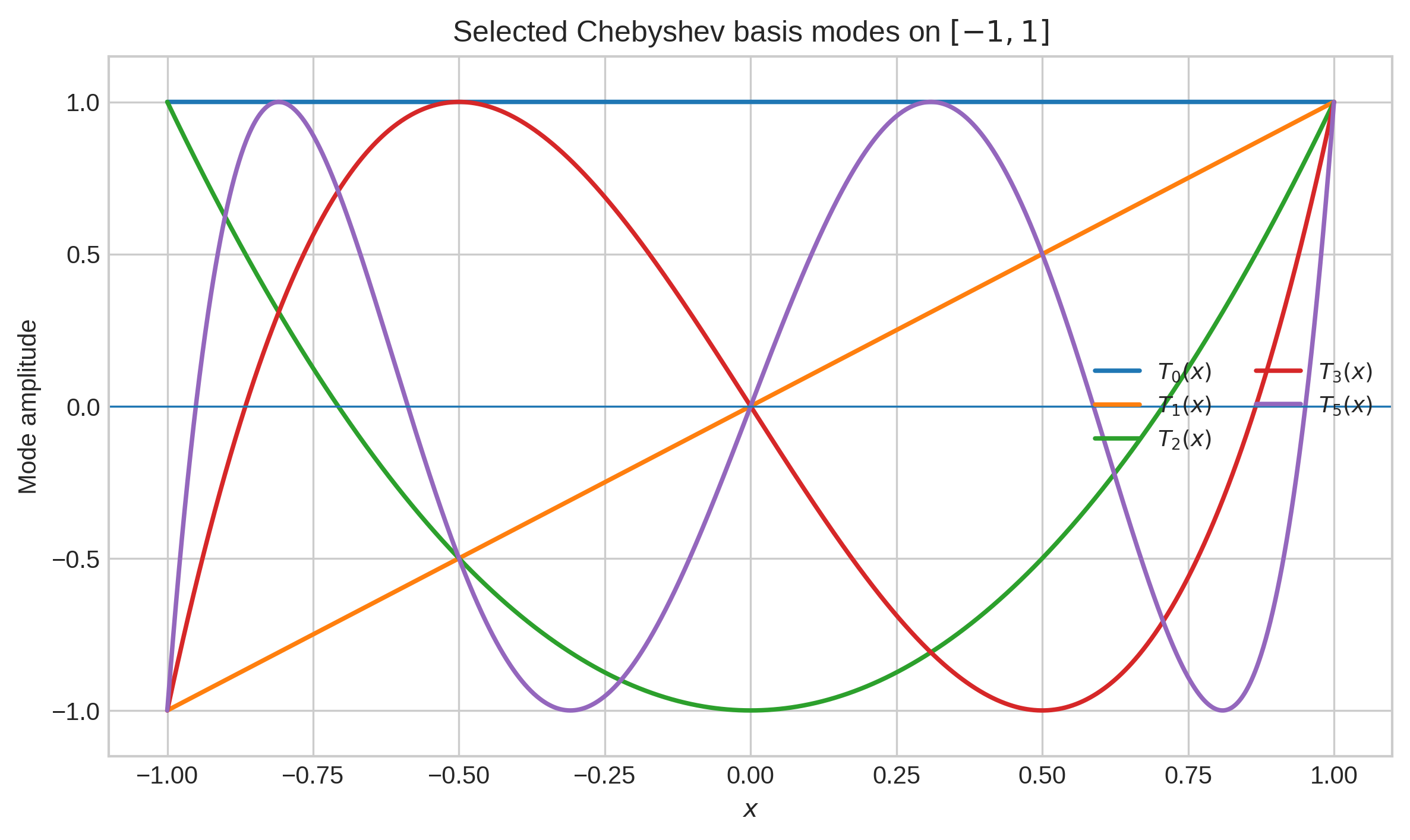
The first five Chebyshev functions can be seen in Figure 1.3.
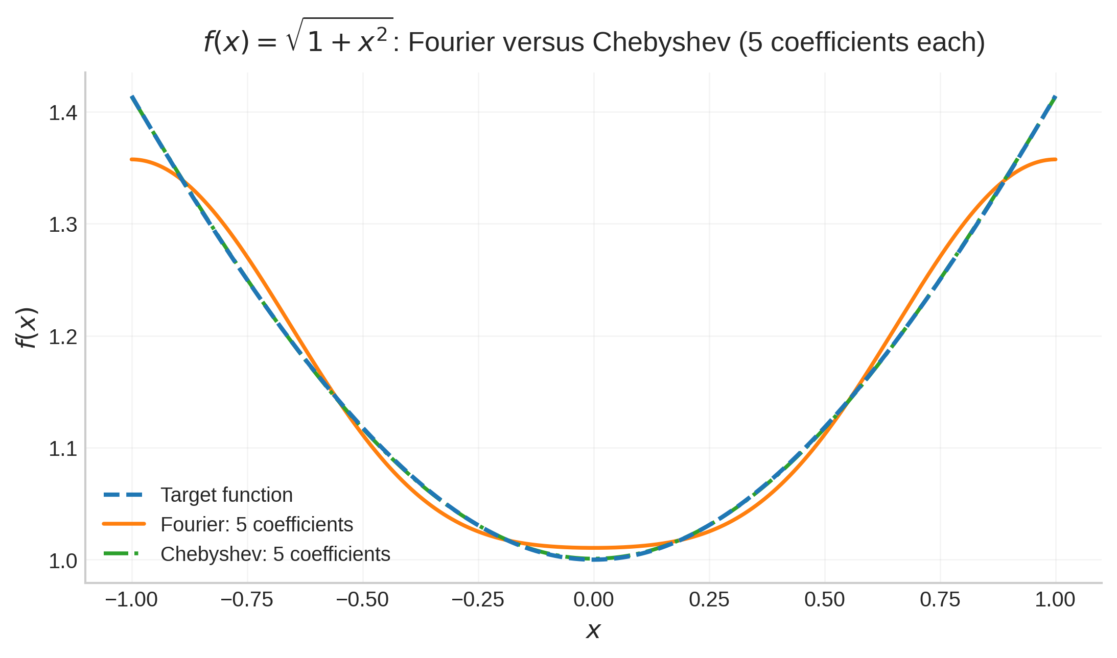
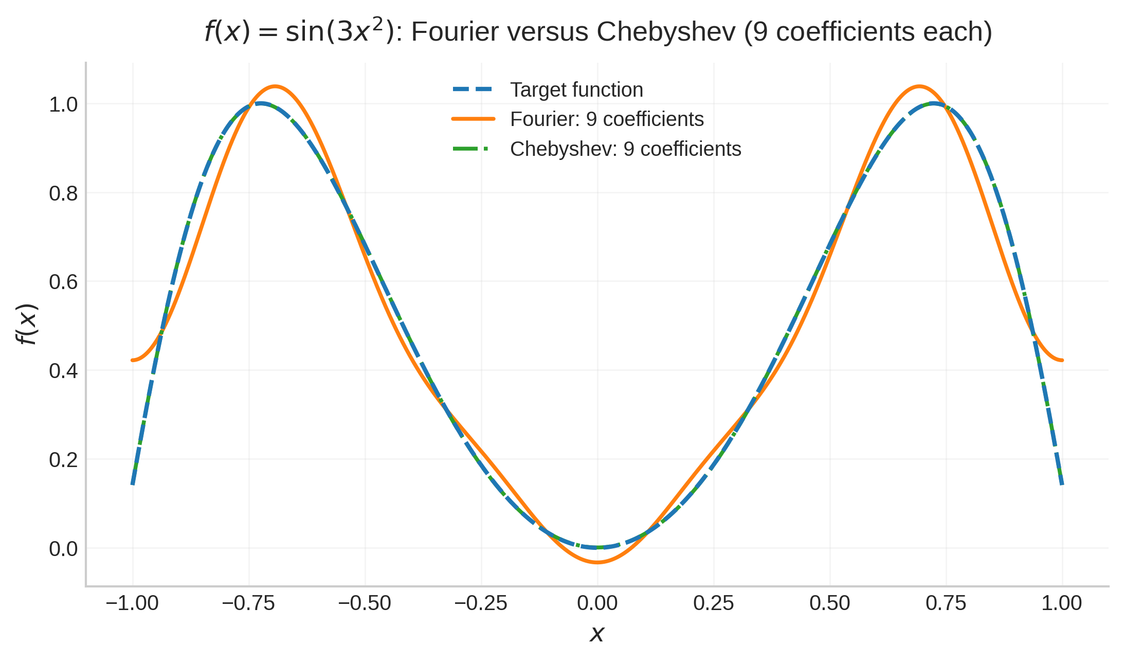
Fourier modes are naturally associated with periodic functions, whereas Chebyshev polynomials are naturally adapted to functions defined on a finite interval. They also have extremely good approximation properties, and relatively few Chebyshev modes can often give an accurate representation of a smooth function.
For this reason Chebyshev expansions are widely used in numerical approximation and particularly in spectral methods for differential equations.
Two example comparisons between the Fourier and Chebyshev series are shown in Figure 1.4, which are both examples seen for the Fourier approximation shown in Figure 1.2 (Gaussian and square wave). We see (for the same number of modes in the partial sum) they perform similarly. However in the second two cases, \(\sqrt{1+x^2}\) and \(\sin{3x^2}\), we see the Chebyshev partial sum significantly outperforming the Fourier partial sum.
1.2.2 The general coefficient grab.
In the first half of this course we saw there are lots of bases/coordinate systems which can be used to describe vectors. They are chosen to best fit the nature of the system being considered, for example, planetary dynamics are best described in spherical coordinates. There are lots of other function bases aside from the Fourier series which similarly, depending on the set of functions being considered, can be better adapted to that description. We just saw for example the Chebyshev basis has certain advantages over Fourier from a numerical (approximation) standpoint.
Let’s assume we have some non-zero family of functions \(\psi_n(x)\) \(n=0,1,2,\dots \infty\), and that they are orthogonal with some weight function \(r(x)\) on some domain \(x\in[a,b]\): \[ \left<\psi_n,r(x)\psi_m\right> = 0,\mbox{ if } n \neq m. \] We want to describe some arbitrary function \(f(x)\) on \(x\in[a,b]\), and assume its weighted norm is finite, \(\left<f,r(x)f\right><\infty\). This is the weighted square-integrable space often denoted \(L^2_r([a,b])\). Our aim is then to find coefficients \(a_n\) such that: \[ f(x) = \sum_{n=0}^{\infty}a_n\psi_n(x). \] To get the coefficient \(a_m\) we use the coefficient grab method. We first multiply by the basis function \(\psi_m(x)\) and weight \(r(x)\), then apply the inner product (integrate):
\[\begin{align} f(x)r(x)\psi_m(x) &= \sum_{n=0}^{\infty}a_n\psi_n(x)r(x)\psi_m(x), \\ \langle f(x),r(x)\psi_m \rangle &= \sum_{n=0}^{\infty}a_n \langle\psi_n(x),r(x)\psi_m\rangle = a_m \langle\psi_m(x),r(x)\psi_m\rangle, \end{align}\] where we have imposed linearity of the inner product and orthogonality. Then we have the coefficient formula: \[ a_m = \frac{\langle f(x),r(x)\psi_m\rangle}{\langle\psi_m(x),r(x)\psi_m\rangle}. \]
Let’s try an example with the Chebyshev basis on \([-1,1]\). Strictly, the Dirac delta is not an \(L^2_r\) function but a distribution; the same projection idea can nevertheless be used to construct its expansion in the distributional sense:
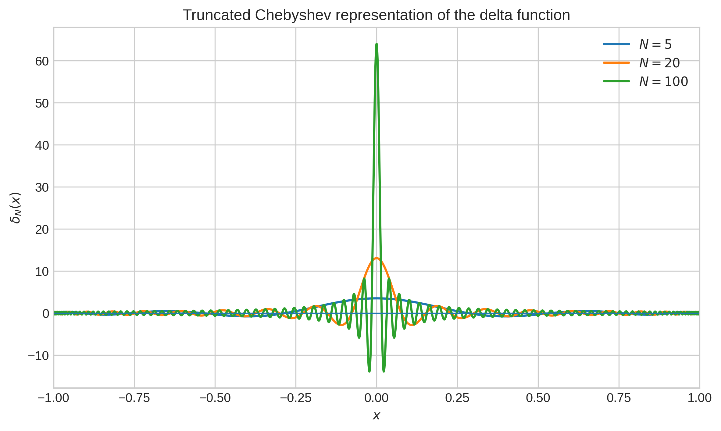
In Figure 1.5 we see plots of the truncated form of this series: \[ \delta_N(x) = \frac{1}{\pi}+\frac{2}{\pi}\sum_{n=1}^{N}(-1)^{n}T_{2n}(x). \] One sees as \(N\) increases the approximation becomes increasingly concentrated around \(x=0\), where it develops a sharper and higher peak. I will show you this in class by increasing the value of \(N\) (it ruins the plots somewhat…). In the limit \(N\rightarrow \infty\) these partial sums do not converge pointwise to an ordinary function; instead they converge to the Dirac delta in the distributional sense. At \(x=0\) the peak diverges to \(\infty\). How can we call this a “function”?
In week 5 we will focus on the \(\delta\) function in much more detail when looking at Green’s method. It is this weird localised spike behaviour which allows it to satisfy its definition: \[ f(0) = \int_{a}^{b}\delta(y)f(y)\mathrm{d}y. \] The delta function (distribution) is one of the most crucial and elemental objects in applied mathematics and mathematical physics, allowing us to represent an idealised point source, impulse, or perfectly localised input.
Quantum states are an example of a mode decomposition of a system where the inner product and norm have a physical meaning. We work through a relatively strightforward example in quesiton 6 of the week 5 problem sheet.
1.2.3 Why orthogonality matters: independent components
We have just seen that if the function basis \(\left\{\psi_n(x)\right\}_{n=0}^{\infty}\) are orthogonal (with weight \(r(x)\)), then we can grab each coefficient separately:
\[ a_n = \frac{\left<f,r(x)\psi_n\right>} {\left<\psi_n,r(x)\psi_n\right>}. \]
This is more important than simply giving us a convenient formula for the coefficients. Orthogonality also guarantees linear independence.
To see this, suppose that some finite combination of orthogonal functions is zero,
\[ \sum_{n=0}^{N}c_n\psi_n(x)=0. \]
Taking the weighted inner product with \(\psi_m\) gives
\[ \sum_{n=0}^{N} c_n\left<\psi_n,r(x)\psi_m\right> = c_m\left<\psi_m,r(x)\psi_m\right> =0. \]
Since \(\psi_m\) is non-zero,
\[ \left<\psi_m,r(x)\psi_m\right> > 0, \]
and hence
\[ c_m=0. \]
As this is true for every \(m\), all of the coefficients must vanish. Thus an orthogonal collection of non-zero functions is linearly independent.
It means that the different basis functions describe genuinely separate components of the function. One component cannot be recreated by combining the others.
This is the fundamental idea behind the use of function expansions in this course: we describe a complicated function by the behaviour of many simple, independent functions.
Part 1: independence lets the dynamics separate.
Later, when we study partial differential equations, this becomes extremely powerful. We will write a solution in the form
\[ u(x,t)=\sum_{n=0}^{\infty}c_n(t)y_n(x). \]
For an appropriate linear PDE, substitution will lead to an expression of the form
\[ \sum_{n=0}^{\infty}F_n(t)y_n(x)=0. \]
Because the functions \(y_n(x)\) are orthogonal (and hence independent), we can isolate each component by taking the weighted inner product with \(y_m\):
\[ \left<\sum_{n=0}^{\infty}F_n(t)y_n,r(x)y_m\right> = F_m(t)\left<y_m,r(x)y_m\right> =0. \]
Since \(\left<y_m,r(x)y_m\right>>0\), it follows that
\[ F_m(t)=0, \]
for every \(m\), giving us a separate ordinary differential equation for each coefficient \(c_m(t)\).
So, schematically,
\[ \boxed{ \text{one PDE for a complicated function} \quad\longrightarrow\quad \text{ODEs for simple independent components}. } \]
This is one of the main reasons function-basis expansions are so useful in applied mathematics.
Part 2: independence lets complexity separate.
There is another, more fundamental, reason that these function expansions are so important in analysis.
The space \(L^2([a,b])\) contains an enormous variety of functions. They need not be smooth; they may have sharp peaks, corners, discontinuities, or extremely complicated behaviour. Yet we can represent these complicated objects using sums of very simple functions. For example, Fourier modes
\[ 1,\qquad \sin(nx),\qquad \cos(nx) \]
are infinitely differentiable, as are many of the other basis functions we shall encounter.
Thus we can write schematically
\[ \sum_n \text{coefficient} \times \text{simple function}. \]
So a function which is itself difficult to understand directly can be encoded by a sequence of numbers,
\[ f(x) \quad\longleftrightarrow\quad {a_0,a_1,a_2,\ldots}, \]
describing how much of each simple component it contains.
The importance of linear independence is that these components carry genuinely separate information. We can therefore study the behaviour of the mathematically convenient individual modes, or of their coefficients, rather than always having to confront the full complicated function at once.
This idea is fundamental throughout mathematical analysis.
1.2.4 A subtlety: an infinite-dimensional basis
There is, however, an important difference between this argument and ordinary finite-dimensional linear algebra.
For a finite-dimensional basis, linear independence is enough to guarantee that a representation is unique. If
\[ \sum_{n=0}^{N}a_n\psi_n = \sum_{n=0}^{N}b_n\psi_n, \]
then
\[ \sum_{n=0}^{N}(a_n-b_n)\psi_n=0, \]
and linear independence immediately gives \(a_n=b_n\).
For an infinite expansion,
\[ f(x)=\sum_{n=0}^{\infty}a_n\psi_n(x), \]
there is more to establish. We need to know what we mean by convergence of the infinite series and, crucially, that our collection of functions is complete: there must not be functions in our function space which cannot be constructed from these modes.
Regular Sturm–Liouville theory provides an important and very general setting in which this completeness can be proved. Closely related completeness results also apply to other standard systems such as Fourier and Chebyshev expansions.
You are not expected to understand the details of the theorem below yet, and you do not need to know or reproduce its proof for this course. For now, the key word is complete: the theorem tells us that the eigenfunctions provide enough independent modes to represent every function in the relevant function space.
We will return to Sturm–Liouville theory later and explain where these problems come from and why this result is so useful. A supplementary discussion of the proof will be provided separately for those who are interested; it is not part of the examinable material.
Theorem 1.1 (Sturm–Liouville completeness theorem) Consider the weighted Sturm–Liouville eigenvalue problem
\[ Ly=\lambda r(x)y, \]
where
\[ Ly= \frac{\mathrm{d}}{\mathrm{d}x} \left( p(x)\frac{\mathrm{d}y}{\mathrm{d}x} \right) +q(x)y, \qquad a\leq x\leq b, \]
with separated homogeneous boundary conditions
\[ \alpha_1y(a)+\alpha_2y'(a)=0, \]
\[ \alpha_3y(b)+\alpha_4y'(b)=0. \]
For a regular Sturm–Liouville problem, the eigenfunctions
\[ y_0(x),y_1(x),y_2(x),\ldots \]
form a complete orthogonal set with weight \(r(x)\).
Thus, for any
\[ f\in L^2_r([a,b]), \qquad \int_a^b |f(x)|^2r(x)\,\mathrm{d}x<\infty, \]
we can write, with convergence in the weighted \(L^2\) sense,
\[ f(x)=\sum_{n=0}^{\infty}c_ny_n(x), \]
where the coefficients are uniquely determined by
\[ c_n= \frac{ \displaystyle\int_a^b f(x)y_n(x)r(x)\,\mathrm{d}x }{ \displaystyle\int_a^b y_n^2(x)r(x)\,\mathrm{d}x }. \]
The completeness part of this theorem is much deeper than the finite-dimensional linear-independence argument above. A rigorous proof requires us to make precise the convergence of the infinite expansion and then show that there can be no non-zero function in \(L^2_r([a,b])\) which is orthogonal to every eigenfunction. Classical proofs make use of deeper results about approximation and convergence of functions.
We will not prove this theorem here. I have compiled a document which outlines the proof which is on the ultra webpage in the lecture notes section. It relies on some fudnamental theorems of approximation.
We will return to Sturm–Liouville theory later in the course, where we will see why this particular class of eigenvalue problems is so general, why it appears naturally in many physical problems, and why its orthogonal and complete eigenfunctions are so useful. You will see critical aspects of the full proof then.
There are therefore three ingredients working together:
- Orthogonality lets us isolate each coefficient.
- Orthogonality implies linear independence, so the modes describe genuinely separate components.
- Completeness tells us that there are enough of these independent components to represent every function in the relevant function space.
Together these allow us to replace the behaviour of one complicated function by the behaviour of many much simpler components.
1.2.5 Extension to higher dimensions
Everything we have discussed extends naturally to functions of several spatial variables.
Let
\[ \mathbf{x}=(x_1,x_2,\ldots,x_n)\in D\subset\mathbb{R}^n, \]
and consider functions \(u(\mathbf{x})\) and \(v(\mathbf{x})\) defined on \(D\).
The inner product is
\[ \langle u,v\rangle = \int_D u(\mathbf{x})v(\mathbf{x}) \,\mathrm{d}^n\mathbf{x}, \]
The corresponding weighted norm is
\[ \|u\|^2 = \langle u,r(\mathbf{x})u\rangle = \int_D r(\mathbf{x})|u(\mathbf{x})|^2 \,\mathrm{d}^n\mathbf{x}. \]
where \(r(\mathbf{x})>0\) is an appropriate weight function.
Exactly as in one dimension, two functions are orthogonal with weight \(r(\mathbf{x})\) if
\[ \langle u,rv\rangle=0. \]
Suppose we have a complete set of orthogonal basis functions
\[ \left\{ \Phi_{\mathbf{k}}(\mathbf{x}) \right\}, \]
where
\[ \mathbf{k}=(k_1,k_2,\ldots,k_n) \]
is a collection of integers labelling a particular mode.
A function can then be expanded as
\[ f(\mathbf{x}) = \sum_{\mathbf{k}} a_{\mathbf{k}}\Phi_{\mathbf{k}}(\mathbf{x}). \]
The important point is that the coefficient grab is exactly the same as in one dimension:
\[ \boxed{ a_{\mathbf{k}} = \frac{ \langle f,r(\mathbf{x})\Phi_{\mathbf{k}}\rangle }{ \langle\Phi_{\mathbf{k}},r(\mathbf{x})\Phi_{\mathbf{k}}\rangle }. } \]
Nothing fundamental has changed. The functions now depend on several variables, and each mode may require several indices to label it, but orthogonality still allows us to isolate one independent component at a time.
1.2.5.1 Separable bases
For some particularly useful domains the basis functions can be written as products of one-dimensional basis functions.
For example, suppose
\[ D=[a_1,b_1]\times[a_2,b_2]\times\cdots\times[a_n,b_n], \]
and the basis functions have the form
\[ \Phi_{\mathbf{k}}(\mathbf{x}) = \psi^{(1)}_{k_1}(x_1) \psi^{(2)}_{k_2}(x_2) \cdots \psi^{(n)}_{k_n}(x_n). \]
If the weight also separates,
\[ r(\mathbf{x}) = r_1(x_1)r_2(x_2)\cdots r_n(x_n), \]
then the inner product of two basis functions separates into a product of one-dimensional inner products:
\[ \left\langle \Phi_{\mathbf{k}}, r(\mathbf{x})\Phi_{\mathbf{m}} \right\rangle = \prod_{j=1}^{n} \left\langle \psi^{(j)}_{k_j}, r_j(x_j)\psi^{(j)}_{m_j} \right\rangle. \]
Hence orthogonality in each coordinate direction produces orthogonality of the multidimensional modes.
In some examples the coefficient integral itself will also separate into products of one-dimensional integrals. This is a very useful simplification, but it is not part of the coefficient grab itself: the general formula is always
\[ a_{\mathbf{k}} = \frac{ \langle f,r(\mathbf{x})\Phi_{\mathbf{k}}\rangle }{ \langle\Phi_{\mathbf{k}},r(\mathbf{x})\Phi_{\mathbf{k}}\rangle }. \]
Fourier series on rectangular domains provide a simple and important example of such a separable basis, which we consider next.
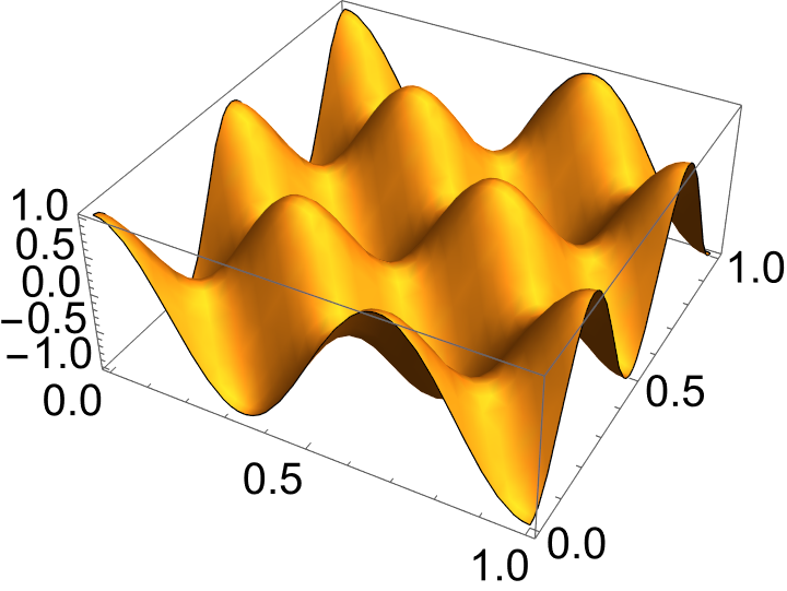
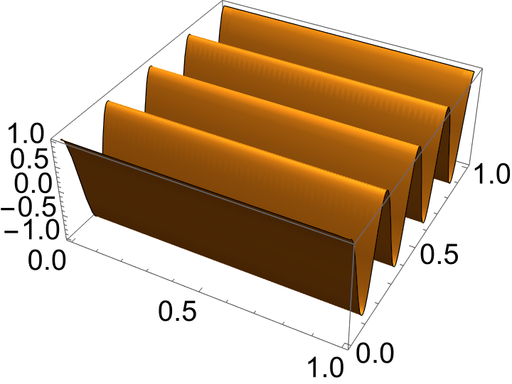
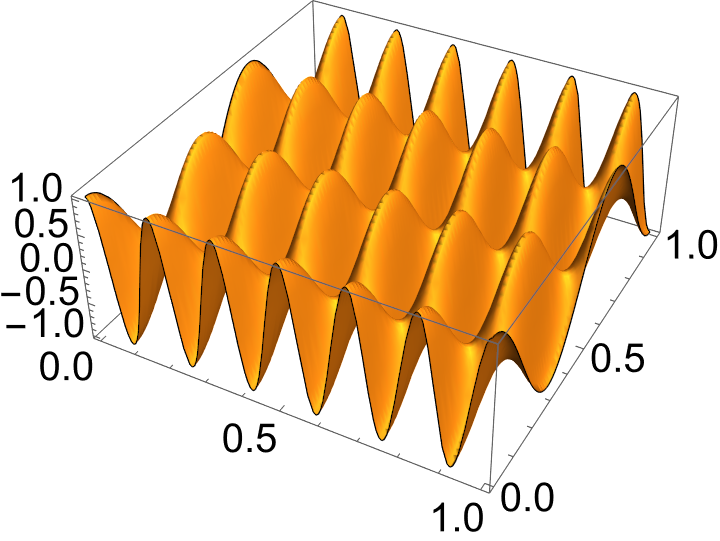
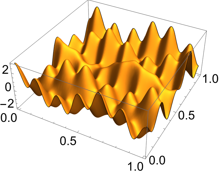
Figure Figure 1.6 shows examples of two-dimensional Fourier product modes and their superposition. Depending on the symmetry of \(f(x,y)\), a Fourier expansion may involve cosine–cosine, sine–sine, or mixed sine–cosine modes.
For example, a cosine–cosine expansion has the form
\[ f(x,y) = \sum_{m=0}^{\infty} \sum_{n=0}^{\infty}a_{mn}\cos\left(\frac{m\pi x}{L_x}\right)\cos\left(\frac{n\pi y}{L_y}\right). \]
The coefficient grab works in exactly the same way for all of these combinations. Let us see it in action in two explicit examples:
I want you to see an example of the coefficient grab in action in higher dimensions. The actual calculations are very fiddly; basically there is no way round this, but it’s not the kind of thing I would want you to do in an exam. To be clear, I would ask you to write down the explicit integral form of a coefficient; I would not ask you to evaluate all of these integrals.
Question 2 of the week 5 problem set is a 2D Fourier example.
Question 7 of the week 5 problem sheet concerns the two dimensional Legendre transformation.
The important point
Nothing fundamentally new happens: a complicated multidimensional function is still represented as a sum of simple independent modes.
What changes is the geometry. On rectangular domains product bases are natural; on other geometries different bases may be more appropriate – for example, spherical harmonics on a sphere.
We will return to multidimensional expansions later when solving partial differential equations.
By this point you should understand the main ideas behind mode decompositions of functions:
A complicated function can be represented as a sum of simpler basis functions, which we will often call modes.
Orthogonality gives us a way of isolating individual components using the inner product — the coefficient grab.
Orthogonal non-zero basis functions are linearly independent, so each coefficient describes genuinely separate information about the function.
Function spaces such as \(L^2([a,b])\) are infinite-dimensional analogues of vector spaces, with inner products and norms playing the role of dot products and lengths.
Fourier modes are only one possible family of modes. Other bases, such as the Chebyshev polynomials, can be better adapted to different domains, geometries, or kinds of behaviour.
In an infinite-dimensional space we also need completeness: there must be enough basis functions to represent every function in the space.
Complicated, non-smooth and highly localised behaviour can emerge from infinite combinations of very simple smooth basis functions.
The independence of the modes allows us to analyse their behaviour separately. This is what will later allow us to turn a PDE into a collection of simpler ODEs for the individual mode amplitudes.