$$ \def\ab{\boldsymbol{a}} \def\bb{\boldsymbol{b}} \def\cb{\boldsymbol{c}} \def\db{\boldsymbol{d}} \def\eb{\boldsymbol{e}} \def\fb{\boldsymbol{f}} \def\gb{\boldsymbol{g}} \def\hb{\boldsymbol{h}} \def\kb{\boldsymbol{k}} \def\nb{\boldsymbol{n}} \def\tb{\boldsymbol{t}} \def\ub{\boldsymbol{u}} \def\vb{\boldsymbol{v}} \def\xb{\boldsymbol{x}} \def\yb{\boldsymbol{y}} \def\Ab{\boldsymbol{A}} \def\Bb{\boldsymbol{B}} \def\Cb{\boldsymbol{C}} \def\Eb{\boldsymbol{E}} \def\Fb{\boldsymbol{F}} \def\Jb{\boldsymbol{J}} \def\Lb{\boldsymbol{L}} \def\Rb{\boldsymbol{R}} \def\Ub{\boldsymbol{U}} \def\xib{\boldsymbol{\xi}} \def\evx{\boldsymbol{e}_x} \def\evy{\boldsymbol{e}_y} \def\evz{\boldsymbol{e}_z} \def\evr{\boldsymbol{e}_r} \def\evt{\boldsymbol{e}_\theta} \def\evp{\boldsymbol{e}_r} \def\evf{\boldsymbol{e}_\phi} \def\evb{\boldsymbol{e}_\parallel} \def\omb{\boldsymbol{\omega}} \def\dA{\;d\Ab} \def\dS{\;d\boldsymbol{S}} \def\dV{\;dV} \def\dl{\mathrm{d}\boldsymbol{l}} \def\rmd{\mathrm{d}} \def\bfzero{\boldsymbol{0}} \def\Rey{\mathrm{Re}} \def\Real{\mathbb{R}} \def\grad{\boldsymbol\nabla} \newcommand{\dds}[2]{\frac{d{#1}}{d{#2}}} \newcommand{\ddy}[2]{\frac{\partial{#1}}{\partial{#2}}} \newcommand{\pder}[3]{\frac{\partial^{#3}{#1}}{\partial{#2}^{#3}}} \newcommand{\deriv}[3]{\frac{d^{#3}{#1}}{d{#2}^{#3}}} \newcommand{\ddt}[1]{\frac{d{#1}}{dt}} \newcommand{\DDt}[1]{\frac{\mathrm{D}{#1}}{\mathrm{D}t}} \newcommand{\been}{\begin{enumerate}} \newcommand{\enen}{\end{enumerate}}\newcommand{\beit}{\begin{itemize}} \newcommand{\enit}{\end{itemize}} \newcommand{\nibf}[1]{\noindent{\bf#1}} \renewcommand{\vec}{\mathbfit} \def\bra{\langle} \def\ket{\rangle} \renewcommand{\S}{{\cal S}} \newcommand{\wo}{w_0} \newcommand{\wid}{\hat{w}} \newcommand{\taus}{\tau_*} \newcommand{\woc}{\wo^{(c)}} \newcommand{\dl}{\mbox{$\Delta L$}} \newcommand{\upd}{\mathrm{d}} \newcommand{\dL}{\mbox{$\Delta L$}} \newcommand{\rs}{\rho_s} $$
5.1 Motivation for Green’s method
In this section we will devise an alternative approach to viewing and solving linear BVP’s, using the so-called Green’s function. Along the way we will encounter one of the most fundamental “functions” in mathematics, the Dirac delta function. The understanding of this mathematical object is critical in many fields of mathematics.
5.1.1 Form of the eigenfunction expansion solution
Consider the form of the final solution obtained through the eigenfunction expansion approach. Here we take the unweighted case \(r=1\) and use the sign convention \[ Ly_k=-\lambda_k y_k. \] With a little rearranging we can write the eigenfunction expansion solution found in the previous chapter as: \[ y(x) = -\sum_{k=1}^\infty \frac{\langle f, w_k \rangle}{\lambda_k \langle y_k, w_k \rangle}y_k(x). \]
This requires all \(\lambda_k\neq0\). If zero is an eigenvalue, the Fredholm condition requires \[ \langle f,w\rangle=0 \qquad\text{for every }w\in\ker(L^*). \] If this condition fails for any such \(w\), the boundary value problem has no solution. If it holds, and the homogeneous problem has a non-trivial kernel, the solution is not unique because we can add any homogeneous solution. In the one-dimensional zero-mode case this reduces to the two possibilities discussed in the previous chapter. This observation is directly linked to the Fredholm alternative.
Let’s assume this is not an issue for now. Let \(n_k = \langle y_k, w_k \rangle\) (normalisation), then: \[\begin{eqnarray*} y(x) &=& -\sum_{k=1}^\infty \frac{1}{\lambda_k n_k} \left(\int_a^b f(t) w_k(t) \mathrm{d} t \right)y_k(x)\\ &=& \int_a^b \left( -\sum_{k=1}^\infty \frac{1}{\lambda_k n_k} w_k(t) y_k(x) \right)f(t) \mathrm{d} t\\ &=& \int_a^b g(x,t) f(t) \mathrm{d} t \end{eqnarray*}\] where \[ g(x,t) = -\sum_{k=1}^\infty \frac{w_k(t) y_k(x)}{\lambda_k n_k}. \tag{5.1}\]
Thus, we have constructed a solution to \(Ly=f\) in the form \[ y(x)=\int_a^bg(x,t)f(t)\;\mathrm{d}t. \tag{5.2}\] The function \(g(x,t)\) is called the Green’s function, and Equation 5.1 is an eigenfunction expansion of \(g(x,t)\).
Of course, if we knew the Green’s function, we would have the solution without any need for the expansion, i.e. no need for the eigenfunctions. The goal in this section is to understand the properties of the GF and how to construct it.
Observe that if \(L = L^*\), then \(w_k = y_k\) and: In this case \(g(x,t)=g(t,x)\), and we have the important connection between a self-adjoint operator and a symmetric Green’s function. This symmetry follows from the completeness and orthogonality of the eigenfunctions of a self-adjoint operator.
5.1.2 Inverse of differential operator
A nice way to think of the Green’s function is in terms of inverting the differential operator. Think about the familiar equation \(\mathbf{A}\vec{x}=\vec{b}\) from linear algebra, to be solved for the unknown vector \(\vec{x}\). The solution is given by \[\vec{x}=\mathbfit{A}^{-1}\vec{b},\] i.e. we find the solution by multiplying the inverse of the linear operator (matrix) by the inhomogeneous term. Once you know the inverse operator, you can solve the problem for any given vector \(\vec{b}\). In the context of BVPs, \(L\) is a differential operator, so it stands to reason that the inverse operator involves integration, hence the form of Equation 5.2. Constructing the Green’s function is analogous to finding the inverse of the matrix, once we have \(g\) we can write down the solution Equation 5.2 for any forcing function \(f(x)\).
There is a much more productive route and direct route than performing an eigenfunction expansion, and it invokes some new and deep mathematics which we want to focus on.
5.1.3 An example
I am going to start with an example Green’s function which at first sight is seemingly pulled out of thin air. In fact in section 3.2 we will see how to construct them, but it is an odd method (at least when first encountered) and relies on the understanding of the properties of the Green’s functions which we aim to build
Consider the BVP: \[ \begin{split} & Ly\equiv-y''=f(x),\,\, 0<x<1\\ &y(0)=y(1)=0 \end{split} \] We will temporarily magic the Green’s function out of thin air. \[ g(x,\xi)=\left\{\begin{array}{ll} (1-\xi)x\quad&0<x<\xi\\ (1-x)\xi\quad&\xi<x<1. \end{array}\right. \]
Let’s check this, to do so we use the Leibniz rule for differentiating integrals: \[ \frac{\mathrm{d}}{\mathrm{d}x}\int_{a(x)}^{b(x)}f(x,\xi)\mathrm{d}\xi = \int_{a(x)}^{b(x)}\frac{\partial f(x,\xi)}{\partial x}\mathrm{d}\xi + \frac{\mathrm{d} b(x)}{\mathrm{d}x}f(x,b(x)) - \frac{\mathrm{d} a(x)}{\mathrm{d} x}f(x,a(x)). \]
The following properties regarding the Green’s function itself are easily checked:
- The GF satisfies \(Lg=0\) if \(x\neq\xi\)
- \(g(x,\xi)\) satisfies the boundary conditions as a function of \(x\). This is because we have homogeneous conditions.
- \(g\) is continuous on the whole interval \([0,1]\)
- \(g\) is differentiable everywhere except at \(x=\xi\), where it suffers a jump in the derivative.
These properties hold for the regular second order linear operators considered here.
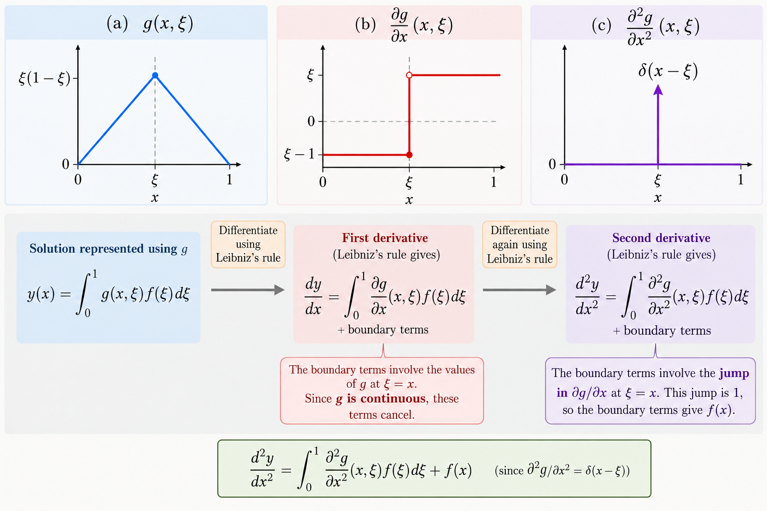
Note, however, that the function \(y(x)\) satisfying \(Ly=f\) is continuously differentiable assuming continuously differentiable \(f\), meaning that the integration with \(f(x)\) smooths out the discontinuity in \(g\). To make sense of this, and to build some physical intuition, we shall need the notion of the delta function. We encountered this object briefly in Chapter 1 if you recall, now we will discuss it and its properties in details.
The idea is illustrated in @#fig-leibniz, we pretend that the Green’s function is something that can be safely differentiated (rather than carefully differentiated by splitting the domain integral as in the above demonstration) i.e. we want to do this:
\[\begin{align} y(x)& = \int_{0}^{1}g(x,\xi)f(\xi)\mathrm{d}\xi,\\ \frac{\mathrm{d} y}{\mathrm{d} x} &=\int_{0}^{1}\frac{\partial g(x,\xi)}{\partial x}f(\xi)\mathrm{d}\xi,\\ \frac{\mathrm{d}^2 y}{\mathrm{d} x^2} & =\int_{0}^{1}\frac{\partial^2 g(x,\xi)}{\partial x^2}f(\xi)\mathrm{d}\xi \end{align}\]
As shown in Figure 5.1 it means the first deirvative has to behave like a step function, the continuity of the greens function itself cancels the boundary terms to allow this. Then the second derivative must somehow act like a point function, zero everywhere except at a single point which just returns the function. The jump in the step function allows the boundary terms to do this.
For this to be a solution we need some “function” \(\delta(x-\xi)\) satisfying \[ \int_{0}^1\delta(x-\xi)f(\xi)\mathrm{d} \xi = f(x),\quad -\frac{\partial^2 g(x,\xi)}{\partial x^2} = \delta(x-\xi). \] We will come to call this the Green’s equation (actually it will later have total derivatives not partial ones).
We expect its first derivative should look (at least locally) like the step (Heaviside) function.
But we should be (initially) skeptical the first derivative of the Green’s function is a step function, it doesn’t have a well defined derivative in the usual sense you saw in Analysis I last year. So how can this \(\delta\) exist?
5.2 Green’s function via delta function
To fix the context, consider stationary heat conduction in a rod:
\[ -y''(x)=f(x)\quad 0<x<1,\quad y(0)=0,\;\; y(1)=0 \]
where \(y(x)\) is the temperature field and \(f(x)\) is a given heat source density.
5.2.1 Delta function
The function \(f(x)\) describes any heat added or removed from the system by the outside world. As a simple scenario, consider a point heat source, say located at the middle of the rod. Physically, this would correspond to applying heat at a single point only. How would we describe such a situation mathematically? What should we use for the function \(f(x)\)?
The notion of a point source is described by the delta function \(\delta\). The most useful way to define it is by what it does when integrated against another function. For a point source located at \(x=a\), we define \(\delta(x-a)\) by
\[ \boxed{ \int_{-\infty}^{\infty}\delta(x-a)f(x)\,\mathrm{d}x=f(a) } \tag{5.3}\]
for every continuous function \(f\) in the class we are considering.
This equation is the definition of the delta function for us. We do not define \(\delta\) by trying to assign it an ordinary value at each point. It is defined by its action on any continuous function \(f\): under an integral, it picks out the value of \(f\) at the point where the delta is located.
This immediately captures the idea of a point source. The delta is concentrated entirely at \(x=a\), and has unit strength. In particular, taking \(f(x)=1\) gives
\[ \int_{-\infty}^{\infty}\delta(x-a)\,\mathrm{d}x=1. \]
Also, if \(f\) vanishes in a neighbourhood of \(a\), then the defining integral is zero. This motivates the familiar shorthand
\[ \delta(x-a)=0\qquad\text{for }x\neq a, \]
but this should be understood as a statement about where the delta is concentrated, rather than as an ordinary pointwise definition.
The problem is that no classical integrable function behaves in this way. A function which is non-zero only at one point either integrates to zero, or is not an ordinary integrable function at all. So the delta function is a different kind of mathematical object, defined through its action under an integral.
5.2.2 Approximating the delta function
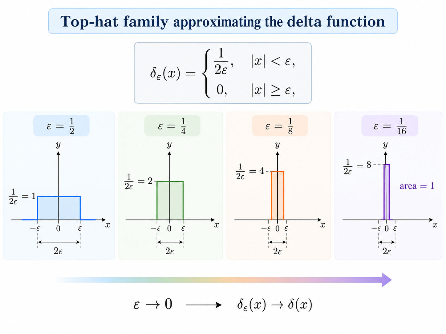
One way to make this less mysterious is to approximate the delta by a sequence of ordinary functions which become increasingly narrow while keeping total area one.
For example, consider the ``top-hat’’ functions
\[ f_n(x)=\left \{ \begin{array}{cc} 0\quad &\text{for } \left\vert x\right\vert>1/n\\ n/2\quad &\text{for } \left\vert x\right \vert \leq 1/n. \end{array}\right. \tag{5.4}\]
Each satisfies
\[ \int_{-\infty}^{\infty}f_n(x)\,\mathrm{d}x=1, \]
and for every fixed \(x\neq0\), this is illustrated in Figure 5.2.
\[ f_n(x)\rightarrow0 \qquad\text{as }n\rightarrow\infty. \]
But this pointwise behaviour is not what defines the delta. What matters is what happens when these functions act on an arbitrary continuous function \(f\).
Let \(F(x)=\int^x f(s)\,\mathrm{d}s\). Then, for a source located at \(x=a\),
\[\begin{align} \lim_{n\rightarrow\infty} \int_{-\infty}^{\infty}f_n(x-a)f(x)\,\mathrm{d}x &= \lim_{n\rightarrow\infty} \int_{a-1/n}^{a+1/n}\frac{n}{2}f(x)\,\mathrm{d}x\\ &= \lim_{n\rightarrow\infty} \frac{F(a+1/n)-F(a-1/n)}{2/n}\\ &= F'(a)=f(a). \end{align}\]
So the top-hat sequence approaches the delta precisely in the sense that its action under an integral approaches the defining action Equation 5.3.
The limiting object is therefore characterised by
\[ \int_{-\infty}^{\infty}\delta(x-a)f(x)\,\mathrm{d}x=f(a), \]
not by ordinary pointwise convergence. This is the sense in which we will use the delta function throughout this chapter.
5.2.3 Properties of delta function
The definition Equation 5.3 immediately gives the sifting property: the delta function sifts out the value of a continuous function at a particular point,
\[ \int_{-\infty}^{\infty}\delta(x-a)f(x)\,\mathrm{d}x=f(a). \]
In particular,
\[ \int_{-\infty}^{\infty}\delta(x)f(x)\,\mathrm{d}x=f(0). \]
Our intended use of \(\delta\) only requires it to be defined through expressions of this kind, so this is enough for what follows.
Antiderivative of \(\delta(x)\).
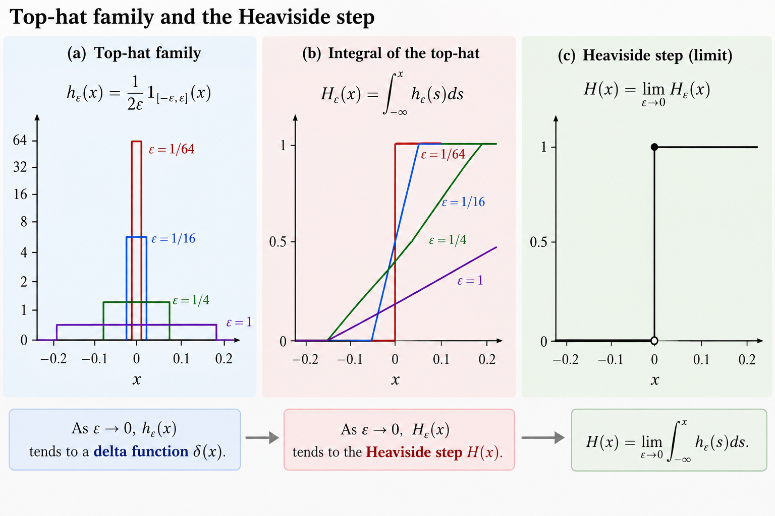
The antiderivative of the delta function is the so-called Heaviside function,
\[ \int_{-\infty}^x \delta(s)\mathrm{d}s= H(x)\equiv\left \{\begin{array}{ll} 0\quad &x<0\\ \frac12\quad &x=0\\ 1\quad &x>0. \end{array}\right. \tag{5.5}\]
The value at \(x=0\) is not important for most applications, but for the symmetric approximating sequence above we obtain \(H(0)=1/2\). Indeed, if
\[ H_n(x)=\int_{-\infty}^x f_n(s)\,\mathrm{d}s, \]
then \(H_n(x)\to H(x)\) as \(n\to\infty\). We leave this detail as an exercise! An illustration of the integral of the top hat family tending to the Heaviside/step function can be found in Figure 5.3.
5.2.4 Point heat source
Let’s return to the heat conduction BVP with a point heat source of unit strength at the centre of the rod:
\[ -y''(x)=\delta(x-1/2), \quad0<x<1 \quad y(0)=y(1)=0. \tag{5.6}\]
Since \(\delta(x-1/2)=0\;\;\forall x\neq1/2\), this implies \[ -y''(x)=0, \quad0<x<1/2,\;1/2<x<1. \tag{5.7}\]
We can easily solve Equation 5.7 in each of the two separate domains \([0,1/2)\) and \((1/2,1]\): \[ y(x) = \left \{\begin{array}{ll} A x +B\quad &x<1/2\\ C x + D \quad &x>1/2.\end{array}\right. \]
and then apply the BC associated with Equation 5.6.
So \(y(0)=0\) implies \(B=0\) and \(y(1)=0\) imples \(D =-C\): \[ y(x) = \left \{\begin{array}{ll} A x \quad &x<1/2\\ C (x - 1) \quad &x>1/2.\end{array}\right. \]
But there are STILL two constants of integration remaining, so we need two more conditions!
As you might expect, since \(\delta(x-1/2)\) has vanished from Equation 5.7, the extra two conditions come in at \(x=1/2\). To derive the extra conditions, imagine integrating equation Equation 5.6 across \(x=1/2\): \[ \int_{1/2-}^{1/2+}-y''(x)\;\mathrm{d}x=\int_{1/2-}^{1/2+}\delta(x-1/2)\;\mathrm{d}x, \] where \(1/2-\) (\(1/2+\)) signifies just to the left (right) of 1/2. Using property Equation 5.3 of the delta function, we have \[ \left[-y'\right]_{1/2-}^{1/2+}=1\quad\Rightarrow\quad y'(1/2+)-y'(1/2-)=-1. \tag{5.8}\] That is, the presence of the delta function defines a jump condition on \(y'\).
Here, \(y(\xi-)=\lim_{x\uparrow \xi}y(x)\), and \(y(\xi+)=\lim_{x\downarrow \xi}y(x)\).
So \[ C - A = -1 \]
and
\[ y(x) = \left \{\begin{array}{ll} A x \quad &x<1/2\\ (A-1)(x -1) \quad &x>1/2.\end{array}\right. \]
If we want to be formal we should only have ever defined our equation inside the integral, then the delta makes sense. It is standard to write the \(\delta\) “naked” with the understanding we will always be integrating it.
The other extra condition needed comes as a requirement that \(y(x)\) is continuous across the point source, that is \[ \left[y\right]_{1/2-}^{1/2+}=0. \tag{5.9}\]
So this requires \[ A/2 = -(A-1)/2, \Rightarrow A=1/2. \]
Thus, all told we have: \[ y(x)=\left\{\begin{array}{ll} \;\;\;\frac{x}{2}\quad&0<x<1/2\\ -\frac{x}{2}+\frac{1}{2}\quad&1/2<x<1. \end{array}\right. \]
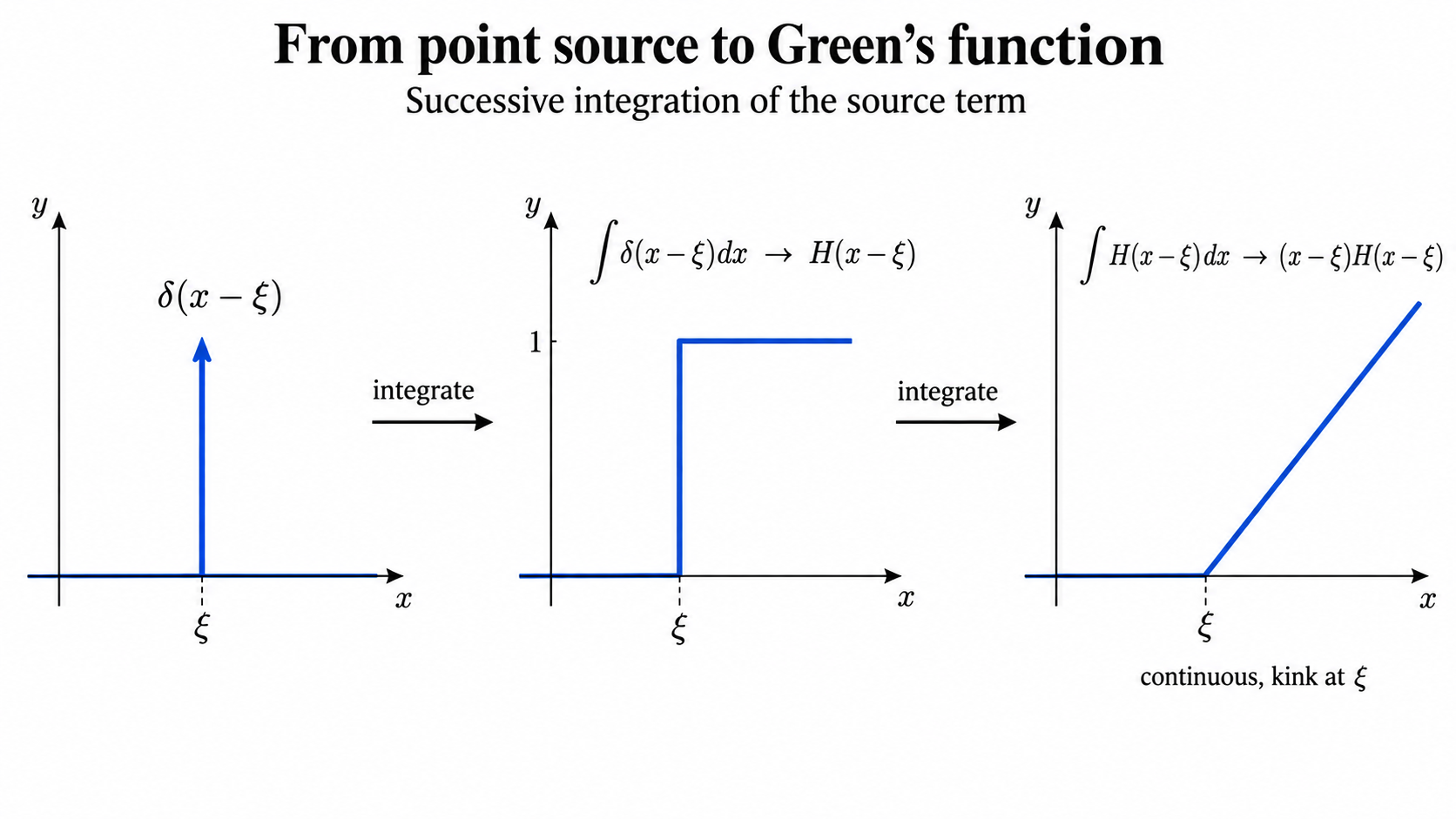
As illustrated in Figure 5.4, the successive integrations around the jump, closed by the jump (delta to Heaviside) and continuity (Heaviside to ramp function), is the opposite of the Leibniz differentiation we saw earlier (illustrated in Figure 5.1). We have reverse engineered our Green’s function with the knowledge of its necessary properties in mind.
Note Figure 5.4 is for an arbitrary source location \(\xi\), everything we did above (i.e the splitting and application of boundary/jump conditions) would have been identical if we had replace \(1/2\) with \(\xi\)…
5.2.5 Green’s function construction
To motivate the construction of the Green’s function, consider the heat conduction problem with an arbitrary heat source:
\[ -y''(x)=f(x), \quad0<x<1,\quad y(0)=y(1)=0. \tag{5.10}\]
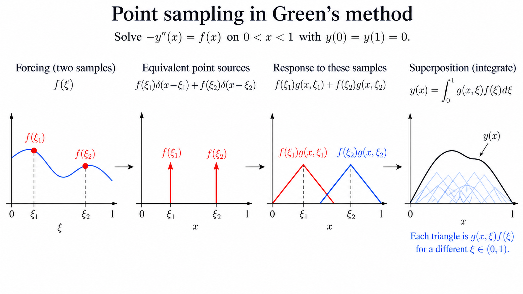
Imagine now describing \(f\) by a distribution of point heat sources with varying strength; that is at point \(x=\xi\) we imagine placing the point source \(f(\xi)\delta(x-\xi)\). We see two such choices in the first two panels of Figure 5.5.
The idea of the Green’s function is to introduce such an extra parameter \(\xi\), and consider the system
\[ -g''(x,\xi)=\delta(x-\xi), \quad0<x<1,\,\,g(0,\xi)=g(1,\xi)=0. \tag{5.11}\]
Note that prime denotes differentiation with respect to \(x\), while \(\xi\) is more like a place-holding variable. So, we have replaced \(f(x)\) by a delta function, in order to solve for the Green’s function \(g(x,\xi)\).
Let’s solve, first on \(x<\xi\) and \(x>\xi\) where we solve the homogeneous equation, \[ -g''(x,\xi)=0. \]
Thus: \[ g(x,\xi) = \left \{\begin{array}{ll} A x +B\quad &x<\xi\\ C x + D \quad &x>\xi.\end{array}\right. \] We basically have the same boundary conditions as above \[ g(x,\xi) = \left \{\begin{array}{ll} A x \quad &x<\xi\\ C (x -1) \quad &x>\xi.\end{array}\right. \]
The jump condition is:
\[ \left[-g'\right]_{\xi-}^{\xi+}=1\quad\Rightarrow\quad g'(\xi+)-g'(\xi-)=-1. \] Thus as before \[ g(x,\xi) = \left \{\begin{array}{ll} A x \quad &x<\xi\\ (A-1)(x -1) \quad &x>\xi.\end{array}\right. \]
Finally we apply continuity: \[ \left[g\right]_{\xi-}^{\xi+}=0. \] Thus \[ A\xi = (A-1)(\xi-1) \]
\[ g(x,\xi)=\left\{\begin{array}{ll} (1-\xi)x\quad&0<x<\xi\\ (1-x)\xi\quad&\xi<x<1. \end{array}\right. \]
These solutions are shown in panel 3 of Figure 5.5 for two example point sources.
This is the solution I showed differentiating correctly at the start of this chapter in sec 3.1.3.
How to get back to the solution of Equation 5.10? For each \(\xi\), the Green’s function gives the solution if a point heat source of unit strength were placed at \(x=\xi\). Conceptually, then, to get the full solution we must add up the point sources, scaled by the value of the heat source at each point: \[ y(x)=\int_0^1g(x,\xi)f(\xi)\;\mathrm{d}\xi. \tag{5.12}\] To verify that this is indeed a solution, we can plug Equation 5.12 into Equation 5.10: \[ -y''(x)=\int_0^1-g''(x,\xi)f(\xi)\;\mathrm{d}\xi=\int_0^1\delta(x-\xi)f(\xi)\;\mathrm{d}\xi=f(x)\;\;\checkmark \]
This sum over all point sources is illustrated in panel 4 of Figure 5.5.
This is the proposed derivative construction I mentioned was on shaky ground in section 3.1.3. It works because the derivative is taken inside the integral \(g\) itself does not need to be classically twice differentiable.
5.3 General linear BVP
We now consider a general \(n\)th order linear BVP with arbitrary continuous forcing function,
\[ Ly(x)=a_ny^{(n)}(x)+a_{n-1}y^{(n-1)}(x)+\dots+a_1y'(x)+a_0y(x)=f(x) \tag{5.13}\] for \(a<x<b\), where the coefficients \(a_i=a_i(x)\) are sufficiently smooth for the differentiations below, and moreover \(a_n(x)\neq0\) \(\forall x\). Along with Equation 5.13 are \(n\) boundary conditions, each a linear combination of \(y\) and derivatives up to \(y^{(n-1)}\), evaluated at \(x=a, b\). For instance, in the case \(n=2\), the general form is:
\[ \begin{split} &BC_1y\equiv \alpha_{11}y(a)+\alpha_{12}y'(a)+\beta_{11}y(b)+\beta_{12}y'(b)=\gamma_1\\ &BC_2y\equiv \alpha_{21}y(a)+\alpha_{22}y'(a)+\beta_{21}y(b)+\beta_{22}y'(b)=\gamma_2. \end{split} \]
5.3.1 General Green’s function
We assume here that the corresponding homogeneous BVP has only the trivial solution, so that the inverse, and hence the Green’s function, exists uniquely. If this fails, the Fredholm conditions discussed previously must be considered.
To solve Equation 5.13 with homogeneous BC \[BC_iy=0,\;\;i=1,\dots,n,\] we first determine the Green’s function by solving
\[ \begin{split} &Lg(x,\xi)=\delta(x-\xi),\quad a<x<b\\ &BC_ig=0. \end{split} \tag{5.14}\]
As before, \[Lg(x,\xi)=\delta(x-\xi)\] implies \[Lg(x,\xi)=0\quad\text{ on }a<x<\xi,\;\;\xi<x<b,\] i.e. we have a homogeneous problem to solve on two separate domains. As before, we require extra conditions, which come by integrating \(Lg(x,\xi)=\delta(x-\xi)\) across \(x=\xi\):
\[ \int_{\xi-}^{\xi^+}\left[a_ng^{(n)}(x,\xi)+\dots+a_0g(x,\xi)\right]\mathrm{d} x=\int_{\xi-}^{\xi^+}\delta(x-\xi)\;\mathrm{d}x. \]
The right hand side clearly integrates to one. If we were to perform an integration by parts on the first term of the left hand side, we would obtain \[ a_n(x)g^{(n-1)}(x,\xi)]_{\xi-}^{\xi+}+\int_{\xi-}^{\xi^+}\left[(a_{n-1}-a_n')g^{(n-1)}+\dots+a_0g(x,\xi)\right]\mathrm{d}x=1. \] This equation is balanced by setting a jump condition on the \((n-1)\)st derivative: \[ \left[g^{(n-1)}(x,\xi)\right]_{\xi-}^{\xi+}=1/a_n(\xi), \] and taking all lower derivatives to be continuous across \(x=\xi\): \[ \left[g^{(j)}(x,\xi)\right]_{\xi-}^{\xi+}=0,\quad j=0,1,\dots n-2. \]
Once the Green’s function is determined, the solution to the BVP is given by \[ y(x)=\int_a^bg(x,\xi)f(\xi)\;\mathrm{d}\xi. \]
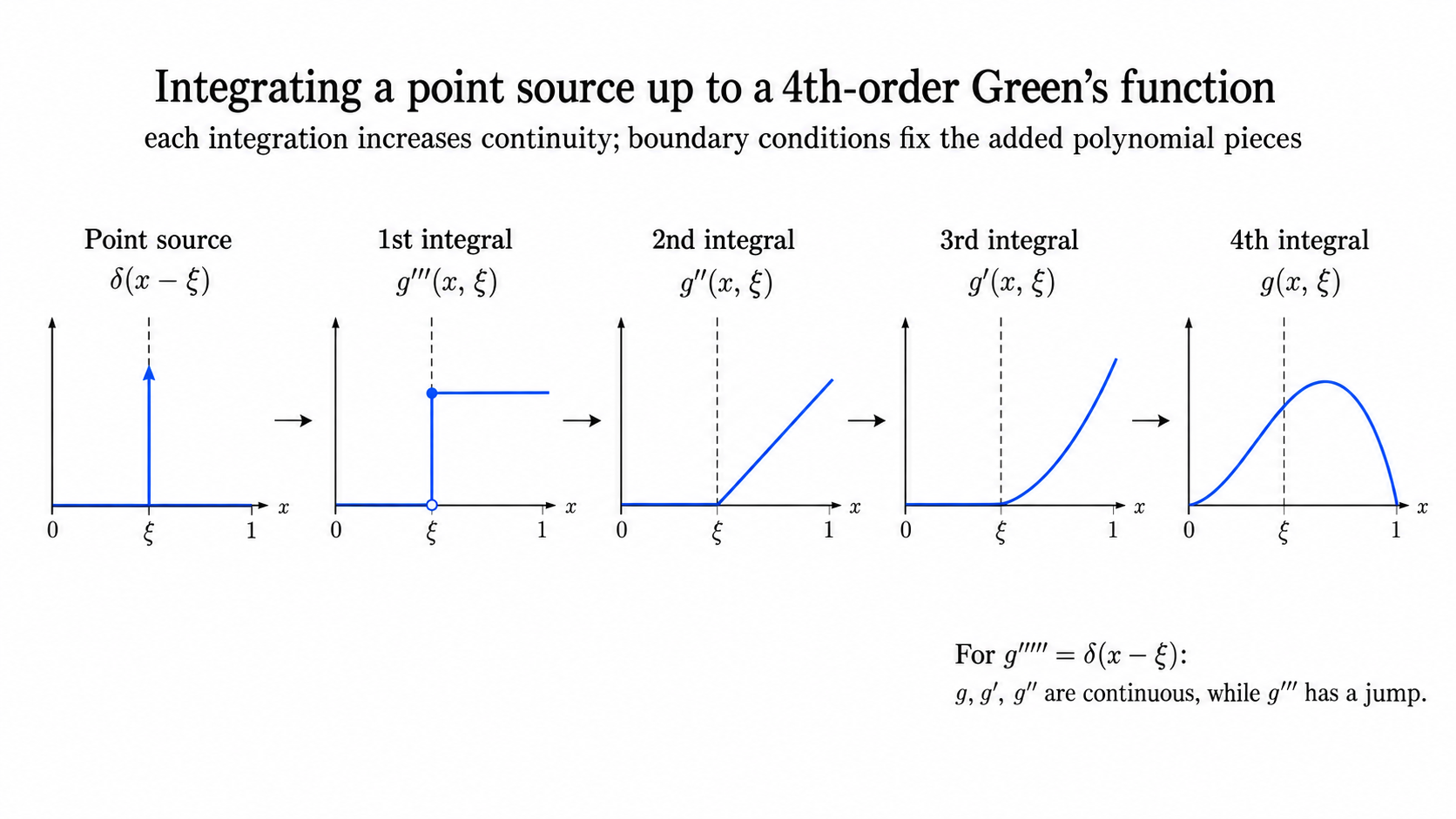
In Figure 5.6 we see a simple higher order example. We have the jump on the \(n-1\)th derivative then continuity there after. The successive integration creates increasingly smooth functions. You can see the full Green’s function has a bump and goes back to zero on its outer boundary. This is not generically true (its not just a result of integrating the delta function)and only results from a Dirichlet Boundary condition, such as we have used in previous examples.
BOUNDARY CONDITIONS MATTER (I think I have mentioned this before right?)
5.4 Three-dimensional Green’s functions in (pretty) arbitrary domains.
We seek \(G(\mathbf{x},\boldsymbol{\xi})\) such that \[ -\nabla_{\mathbf{x}}^2 G(\mathbf{x},\boldsymbol{\xi}) = \delta^{(3)}(\mathbf{x}-\boldsymbol{\xi}), \qquad G(\mathbf{x},\boldsymbol{\xi})\to0 \quad\text{as }|\mathbf{x}|\to\infty. \] Here \(\nabla_{\vec{x}}\) implies the gradient is taken with respect to the \(\vec{x}\) coordinates not \(\boldsymbol{\xi}\), and \(\delta^{(3)}\) is the three-dimensional delta function, characterised by the sifting property \[ \int_{\mathbb R^3} \delta^{(3)}(\mathbf{x}-\boldsymbol{\xi})f(\mathbf{x})\,\mathrm{d}V = f(\boldsymbol{\xi}). \]
By translation and rotational symmetry, \(G\) depends only on the distance \(r=|\mathbf{x}-\boldsymbol{\xi}|\), i.e. \(G(\mathbf{x},\boldsymbol{\xi})=\Phi(r)\) for some radial function \(\Phi\).
Step 1: Solve away from the source.
For \(r>0\) we have \(\nabla_{\mathbf{x}}^2 G=0\), so in spherical coordinates the radial Laplacian gives \[
\Phi''(r)+\frac{2}{r}\,\Phi'(r)=0.
\] Integrating once: \(r^2\Phi'(r)=A\) (constant), hence \(\Phi'(r)=\dfrac{A}{r^2}\) and \[
\Phi(r)=-\frac{A}{r}+B.
\] The decay condition \(G\to0\) as \(r\to\infty\) forces \(B=0\), so for \(r>0\) \[
G(\mathbf{x},\boldsymbol{\xi})
=
\Phi(r)
=
\frac{C}{r}
\quad\text{with }C=-A.
\]
Step 2: Fix the constant by normalization.
Integrate the defining equation over a ball \(B_\varepsilon(\boldsymbol{\xi})\) of radius \(\varepsilon\) centred at \(\boldsymbol{\xi}\) and use the divergence theorem: \[
\int_{B_\varepsilon(\boldsymbol{\xi})}\!\!-\nabla_{\mathbf{x}}^2 G\,\mathrm{d}V
=
\int_{\partial B_\varepsilon(\boldsymbol{\xi})}\!\!-\frac{\partial G}{\partial n}\,\mathrm{d}S
=
\int_{B_\varepsilon(\boldsymbol{\xi})}\!\!\delta^{(3)}(\mathbf{x}-\boldsymbol{\xi})\,\mathrm{d}V
=
1.
\] Since \(G=C/r\), its radial derivative is \(\dfrac{\partial G}{\partial r}=-\dfrac{C}{r^2}\). On the sphere \(|\mathbf{x}-\boldsymbol{\xi}|=\varepsilon\), the outward normal derivative is \(\dfrac{\partial G}{\partial n}=\dfrac{\partial G}{\partial r}=-\dfrac{C}{\varepsilon^2}\), hence \[
\int_{\partial B_\varepsilon(\boldsymbol{\xi})}\!\!-\frac{\partial G}{\partial n}\,\mathrm{d}S
=
\int_{\partial B_\varepsilon(\boldsymbol{\xi})}\!\!\frac{C}{\varepsilon^2}\,\mathrm{d}S
=
\frac{C}{\varepsilon^2}\cdot 4\pi \varepsilon^2
=
4\pi C.
\] Therefore \(4\pi C=1\), so \(C=\dfrac{1}{4\pi}\) and \[
G(\mathbf{x},\boldsymbol{\xi})
=
\frac{1}{4\pi\,|\mathbf{x}-\boldsymbol{\xi}|}.
\]
Uniqueness.
Any other solution differing from \(G\) by a harmonic function vanishing at infinity must be identically zero, so this \(G\) is unique.
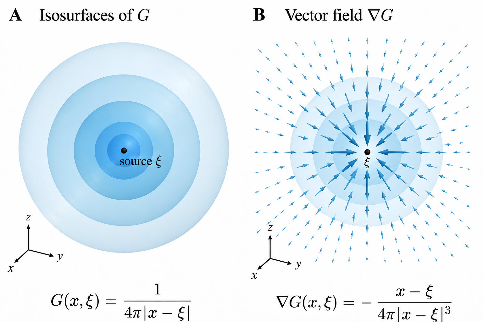
We see in Figure 5.7 the function defines a set of spherical isosurfaces, crucially the vector field \(\nabla G\) acts like a source/sink field radiating away from/towards the source itself (depending on your sign convention).
One of my research interests is vector field topology (entanglement) the Green’s function of the Laplacian in more complex domains plays a key role in this, if time permits I will Rhapsodise on the Greatness of the Green’s function It knows….. But you might be luck and we run short on time….
5.4.1 Arbitrary bounded domain: Green’s representation and boundary integrals (NON EXAMINABLE)
Let \(\Omega\subset\mathbb{R}^3\) be a bounded domain with smooth boundary \(\partial\Omega\).
For \[
-\nabla^2 u(\mathbf{x})=f(\mathbf{x})\quad\text{in }\Omega,
\] it is cleaner to regard the Green’s function as a function of the integration variable \(\boldsymbol{\xi}\), with \(\mathbf{x}\) fixed: \[
-\nabla_{\boldsymbol{\xi}}^2G(\mathbf{x},\boldsymbol{\xi})
=
\delta^{(3)}(\mathbf{x}-\boldsymbol{\xi}).
\] Green’s representation formula (with outward normal \(\vec{n}_{\boldsymbol{\xi}}\) at \(\boldsymbol{\xi}\in\partial\Omega\)) reads \[
u(\mathbf{x})
=
\int_{\partial\Omega}
\left(
G(\mathbf{x},\boldsymbol{\xi})
\frac{\partial u}{\partial n_{\boldsymbol{\xi}}}(\boldsymbol{\xi})
-
u(\boldsymbol{\xi})
\frac{\partial G}{\partial n_{\boldsymbol{\xi}}}(\mathbf{x},\boldsymbol{\xi})
\right)\mathrm{d}S_{\boldsymbol{\xi}}
+
\int_{\Omega}
G(\mathbf{x},\boldsymbol{\xi})f(\boldsymbol{\xi})\,\mathrm{d}V_{\boldsymbol{\xi}},
\] where \(G\) is the Green’s function appropriate to the boundary condition.
Dirichlet problem (\(u=g\) on \(\partial\Omega\)): choose the Dirichlet Green’s function \(G_D\) solving \[ -\nabla_{\boldsymbol{\xi}}^2G_D(\mathbf{x},\boldsymbol{\xi}) = \delta^{(3)}(\mathbf{x}-\boldsymbol{\xi}), \qquad G_D(\mathbf{x},\boldsymbol{\xi})=0 \quad\text{for }\boldsymbol{\xi}\in\partial\Omega. \] Then \[ u(\mathbf{x}) = -\int_{\partial\Omega} g(\boldsymbol{\xi}) \frac{\partial G_D}{\partial n_{\boldsymbol{\xi}}}(\mathbf{x},\boldsymbol{\xi}) \,\mathrm{d}S_{\boldsymbol{\xi}} + \int_{\Omega} G_D(\mathbf{x},\boldsymbol{\xi})f(\boldsymbol{\xi}) \,\mathrm{d}V_{\boldsymbol{\xi}}, \qquad \mathbf{x}\in\Omega. \] Hence \(u\) is obtained from known boundary data \(g\) and the volume source \(f\).
Neumann problem \(\big(\frac{\partial u}{\partial n}=h\) on \(\partial\Omega\big)\): because constants lie in the kernel of the Neumann Laplacian, the Green’s function must be modified. We use the Neumann function \(G_N\) satisfying \[ -\nabla_{\boldsymbol{\xi}}^2G_N(\mathbf{x},\boldsymbol{\xi}) = \delta^{(3)}(\mathbf{x}-\boldsymbol{\xi}) - \frac{1}{|\Omega|}, \qquad \frac{\partial G_N}{\partial n_{\boldsymbol{\xi}}}=0 \quad\text{on }\partial\Omega, \] together with the normalization \[ \int_\Omega G_N(\mathbf{x},\boldsymbol{\xi})\,\mathrm{d}V_{\boldsymbol{\xi}}=0. \] The Neumann problem itself requires the compatibility condition \[ \int_\Omega f\,\mathrm{d}V = -\int_{\partial\Omega}h\,\mathrm{d}S. \] This condition arises fromm the definition of the problem and use of the divegrence theorem (remember \(\nabla^2 = \nabla \cdot \nabla\)).
The solution is determined only up to an additive constant. Writing \[ \bar u=\frac{1}{|\Omega|}\int_\Omega u\,\mathrm{d}V, \] Green’s representation gives \[ u(\mathbf{x})-\bar u = \int_{\partial\Omega} G_N(\mathbf{x},\boldsymbol{\xi})h(\boldsymbol{\xi})\,\mathrm{d}S_{\boldsymbol{\xi}} + \int_\Omega G_N(\mathbf{x},\boldsymbol{\xi})f(\boldsymbol{\xi})\,\mathrm{d}V_{\boldsymbol{\xi}}. \] If we choose the normalization \(\bar u=0\), this gives \(u\) directly.
Remark (arbitrary shapes).
For a general \(\partial\Omega\), \(G_D\) or \(G_N\) is rarely available in closed form. In practice one can write the solution as the known free-space volume potential together with an unknown boundary layer. For example, \[
u(\mathbf{x})
=
\int_\Omega
\frac{f(\boldsymbol{\xi})}{4\pi|\mathbf{x}-\boldsymbol{\xi}|}
\,\mathrm{d}V_{\boldsymbol{\xi}}
+
\int_{\partial\Omega}
\frac{1}{4\pi|\mathbf{x}-\boldsymbol{\xi}|}\,
\sigma(\boldsymbol{\xi})\,\mathrm{d}S_{\boldsymbol{\xi}},
\] or use a double-layer potential for the boundary correction, \[
u(\mathbf{x})
=
\int_\Omega
\frac{f(\boldsymbol{\xi})}{4\pi|\mathbf{x}-\boldsymbol{\xi}|}
\,\mathrm{d}V_{\boldsymbol{\xi}}
+
\int_{\partial\Omega}
\frac{\partial}{\partial n_{\boldsymbol{\xi}}}
\left(
\frac{1}{4\pi|\mathbf{x}-\boldsymbol{\xi}|}
\right)
\mu(\boldsymbol{\xi})\,\mathrm{d}S_{\boldsymbol{\xi}}.
\] The boundary condition is then enforced to obtain an integral equation for \(\sigma\) or \(\mu\) on \(\partial\Omega\). The unknown part of the problem has therefore been reduced to the boundary.
5.5 Summary
Green’s method gives us another way to solve a linear boundary-value problem
\[ \boxed{Ly=f.} \]
Rather than constructing a new eigenfunction expansion every time the forcing \(f\) changes, we first find the Green’s function for the operator and its boundary conditions. We can then write the solution as
\[ \boxed{ y(x)=\int_a^b g(x,\xi)f(\xi)\,\mathrm{d}\xi. } \]
The main ideas are:
- The Dirac delta is defined by its action under an integral: it picks out the value of a continuous function at a point. It gives us a mathematical way to describe a point source.
- The Green’s function is the response to that point source. In one dimension we construct it from \[ L_x g(x,\xi)=\delta(x-\xi), \] together with the boundary conditions, continuity where required, and the appropriate jump condition at \(x=\xi\).
- The integral solution adds up the responses to point sources distributed throughout the domain, each with strength \(f(\xi)\). This is the same superposition principle that underlies our mode expansions.
- A Green’s function can be viewed as the integral kernel of an inverse differential operator. As we saw in Chapter 3, a zero mode can obstruct that inverse: the Fredholm compatibility conditions may need to be satisfied, and solutions may not be unique.
- The method extends beyond the rod. For example, the free-space Green’s function of the three-dimensional operator \(-\nabla^2\) is \[ G(\mathbf{x},\boldsymbol{\xi}) =\frac{1}{4\pi|\mathbf{x}-\boldsymbol{\xi}|}. \] For a bounded domain, the geometry and boundary conditions determine the appropriate Green’s function.
Chapter 1 taught us how to decompose functions into modes; Chapters 2–4 showed how eigenfunctions arise from differential equations and how we use them to solve PDEs. Green’s method gives us a complementary perspective: find the response to one point source, then build the response to any forcing by adding those point-source responses together.