$$ \def\ab{\boldsymbol{a}} \def\bb{\boldsymbol{b}} \def\cb{\boldsymbol{c}} \def\db{\boldsymbol{d}} \def\eb{\boldsymbol{e}} \def\fb{\boldsymbol{f}} \def\gb{\boldsymbol{g}} \def\hb{\boldsymbol{h}} \def\kb{\boldsymbol{k}} \def\nb{\boldsymbol{n}} \def\tb{\boldsymbol{t}} \def\ub{\boldsymbol{u}} \def\vb{\boldsymbol{v}} \def\xb{\boldsymbol{x}} \def\yb{\boldsymbol{y}} \def\Ab{\boldsymbol{A}} \def\Bb{\boldsymbol{B}} \def\Cb{\boldsymbol{C}} \def\Eb{\boldsymbol{E}} \def\Fb{\boldsymbol{F}} \def\Jb{\boldsymbol{J}} \def\Lb{\boldsymbol{L}} \def\Rb{\boldsymbol{R}} \def\Ub{\boldsymbol{U}} \def\xib{\boldsymbol{\xi}} \def\evx{\boldsymbol{e}_x} \def\evy{\boldsymbol{e}_y} \def\evz{\boldsymbol{e}_z} \def\evr{\boldsymbol{e}_r} \def\evt{\boldsymbol{e}_\theta} \def\evp{\boldsymbol{e}_r} \def\evf{\boldsymbol{e}_\phi} \def\evb{\boldsymbol{e}_\parallel} \def\omb{\boldsymbol{\omega}} \def\dA{\;d\Ab} \def\dS{\;d\boldsymbol{S}} \def\dV{\;dV} \def\dl{\mathrm{d}\boldsymbol{l}} \def\rmd{\mathrm{d}} \def\bfzero{\boldsymbol{0}} \def\Rey{\mathrm{Re}} \def\Real{\mathbb{R}} \def\grad{\boldsymbol\nabla} \newcommand{\dds}[2]{\frac{d{#1}}{d{#2}}} \newcommand{\ddy}[2]{\frac{\partial{#1}}{\partial{#2}}} \newcommand{\pder}[3]{\frac{\partial^{#3}{#1}}{\partial{#2}^{#3}}} \newcommand{\deriv}[3]{\frac{d^{#3}{#1}}{d{#2}^{#3}}} \newcommand{\ddt}[1]{\frac{d{#1}}{dt}} \newcommand{\DDt}[1]{\frac{\mathrm{D}{#1}}{\mathrm{D}t}} \newcommand{\been}{\begin{enumerate}} \newcommand{\enen}{\end{enumerate}}\newcommand{\beit}{\begin{itemize}} \newcommand{\enit}{\end{itemize}} \newcommand{\nibf}[1]{\noindent{\bf#1}} \renewcommand{\vec}{\mathbfit} \def\bra{\langle} \def\ket{\rangle} \renewcommand{\S}{{\cal S}} \newcommand{\wo}{w_0} \newcommand{\wid}{\hat{w}} \newcommand{\taus}{\tau_*} \newcommand{\woc}{\wo^{(c)}} \newcommand{\dl}{\mbox{$\Delta L$}} \newcommand{\upd}{\mathrm{d}} \newcommand{\dL}{\mbox{$\Delta L$}} \newcommand{\rs}{\rho_s} $$
3.1 The eigenfunction problem
Chapter 2 led us naturally to two related problems. First, the eigenvalue boundary-value problem \[ Ly_i(x)=\lambda_i r(x)y_i(x), \] and second, the inhomogeneous boundary-value problem \[ Ly=f(x). \] Here \(L\) is a linear differential operator on \(x\in[a,b]\), the boundary conditions are part of the definition of the problem, and \(r(x)>0\) is a weighting function. Our aim is to understand the properties that make eigenfunction expansions work: orthogonality, coefficient formulae, self-adjointness, completeness and solvability.
The absence of the minus sign, compared to the form of eigenfunction equation used in the previous, is just a matter of convenience. Here it will be more convenient notationally to have it be positive and avoid having to track lots of minus signs. None of the conclusions we draw are affected either way.
Here \(y_i\) is an eigenfunction with corresponding eigenvalue \(\lambda_i\). As with the examples already encountered, this is analogous to the linear algebra eigenproblem
\[ \mathbfsfit{A}\vec{x}_i=\lambda_i\vec{x}_i \] where \(\mathbfsfit{A}\) is a matrix and \(\vec{x}_i\) an eigenvector with eigenvalue \(\lambda_i\), and, as we shall see this is reflected in the terminology and concepts we use to explore the properties of the eigenfunction equation.
3.1.1 A short reminder: inner products and weighted orthogonality
Chapter 1 introduced the function-space language we need, so we only recall the pieces used below. Our ordinary inner product is \[ \langle u,v\rangle=\int_a^b u(x)v(x)\,\mathrm{d}x. \]
When a positive weight \(r(x)\) is present we keep it explicitly in the inner product. Thus two functions are orthogonal with weight \(r\) when \[ \langle u,r v\rangle=\int_a^b r(x)u(x)v(x)\,\mathrm{d}x=0. \]
The same notation gives the weighted norm (squared) \[ \langle u,r u\rangle>0 \] for any non-zero \(u\), provided \(r(x)>0\) in the interior of the domain.
The point of Chapter 1 was that orthogonal families let us represent functions mode by mode. In this chapter we ask when the eigenfunctions of a general differential operator have exactly the properties required to act as such a basis.
3.1.2 Adjoint operators
Crucial to almost everything that follows is the notion of the adjoint of an operator. I always find it seems a bit arbitrary when first written down, so first an analogy to the adjoint matrix in the finite dimensional case.
The adjoint matrix For a matrix \(\mathbfsfit{A}=[a_{ij}]\), the adjoint matrix \(A^\dagger\) is defined by \[ (\mathbfsfit{A}^\dagger)_{ij}=a_{ji}. \] That is, \(\mathbfsfit{A}^\dagger\) is obtained by taking the transpose of \(A\). It satisfies: \[ \langle \mathbfsfit{A} \vec{u},\vec{v}\rangle = \langle \vec{u},\mathbfsfit{A}^{\dagger}\vec{v}\rangle \] or more familiarly: \[ \mathbfsfit{A} \vec{u}\cdot \vec{v} = \vec{u}\cdot \mathbfsfit{A}^{\dagger}\vec{v}. \]
For a matrix equation
\[
\mathbfsfit{A}\vec{x}=\vec{b},
\] we know from linear algebra that a solution exists if and only if \[
\vec{b}\perp\ker(A^\dagger),
\] that is, \(\vec{b}\) is orthogonal to all vectors \(\vec{y}\) satisfying \(\mathbfsfit{A}^\dagger\vec{y}=0\). This is the Fredholm alternative for matrices. You likely didn’t hear it called that before, but it is the name of a theorem we will encounter soon, which is a VAST generalisation of this idea.
Often people refer the to matrix of co-factors transposed (used to calculate the inverse) as the adjoint, as opposed ot the definition given above. The martix (of cofactors) sometimes that is called the adjugate matrix. This potential confusion won’t ever be an issue in this course, however.
The adjoint matrix is central to solvability: the equation \(\mathbfsfit{A}\vec{x}=\vec{b}\) can only be solved when \(\vec{b}\) is orthogonal to the nullspace of \(\mathbfsfit{A}^\dagger\).
Now, the operator version
Definition 3.1 For operator \(L\) with BC associated with an inner product \(\langle \rangle\) the adjoint operator (\(L^*\),\(BC^*\)) is defined by the inner product relation: \[ \langle Ly, w \rangle=\langle y, L^*w \rangle. \]
To determine the adjoint, one needs to move the derivatives of the operator from \(y\) to \(w\), and define adjoint boundary conditions so that all boundary terms vanish.
We seek a function \(L^*w\) such that: \[ \int_a^b (w)(y'')\mathrm{d}x = \int_a^b (y)(L^*w)\mathrm{d}x \] To do this, we need to shift the derivatives from \(y\) to \(w\) using integration by parts:
\[\begin{align} \int_a^b wy''\mathrm{d}x & = wy' \vert_a^b - \int_a^b w'y'\mathrm{d}x\\ & = wy' - w'y\vert_a^b +\int_a^b y w'' \mathrm{d}x. \end{align}\]
A comparison of the integral parts suggests: \[ L^*w = \frac{\mathrm{d}^2w}{\mathrm{d}x^2} \Rightarrow L^* = \deriv{}{x}{2}. \] The inner product only includes integral terms, so the boundary terms must vanish, which will define boundary conditions on \(w\), i.e. this defines BC*. Here, we require \[ w(b)y'(b) - w'(b)y(b) - w(a)y'(a) +w'(a)y(a)=0. \] Using the BCs \(y'(b) = 3y(b)\) and \(y(a) = 0\), gives: \[ 0 = y(b)\Big(3w(b) - w'(b)\Big) - w(a)y'(a) +\underbrace{w'(a)y(a)}_{= 0} \] As these terms need to vanish for all values of \(y(b)\) and \(y'(a)\), we can infer two boundary conditions on \(w\):
- \(y(b)\): \(3w(b)-w'(b) = 0\)
- \(y'(a)\): \(w(a) = 0\)
so all told the answer to our problem is:
If \(L=L^*\) and \(BC=BC^*\) then the boundary-value problem is self-adjoint. If the differential expression satisfies \(L=L^*\) but the boundary conditions do not match their adjoint conditions, we call the differential expression formally self-adjoint, but the full boundary-value problem is not self-adjoint.
Some books use the terminology formally self-adjoint for the differential expression and fully self-adjoint when both \(L=L^*\) and \(BC=BC^*\).
Questions 1-3 of the week 8 problem sheet will get you familiar with calculating adjoint operators.
3.2 Eigenfunction properties
To use eigenfunctions as a basis, two properties are particularly important.
Proposition 3.1 For the class of real boundary-value problems considered here, the adjoint eigenproblem has the same eigenvalues as the original problem.
That is, if \[ Ly=\lambda r(x)y, \] then there is a corresponding adjoint eigenfunction problem \[ L^*w=\lambda r(x)w. \]
Proof. The adjoint is defined by \[ \langle Lv,w\rangle=\langle v,L^*w\rangle \] for admissible functions \(v\). For an eigenvalue \(\lambda\) we seek the corresponding adjoint eigenfunction with the same value of \(\lambda\). Using \[ Lv=\lambda r(x)v \] in the adjoint identity gives \[ \langle v,L^*w\rangle = \langle Lv,w\rangle = \langle \lambda r(x)v,w\rangle = \langle v,\lambda r(x)w\rangle. \] Thus the corresponding adjoint eigenproblem is \[ \boxed{ L^*w=\lambda r(x)w. } \]
Proposition 3.2 Eigenfunctions corresponding to different eigenvalues are orthogonal to each other’s adjoint (under a weighted inner product).
That is, if \[ Ly_j=\lambda_j r(x)y_j,\qquad L^*w_j=\lambda_j r(x)w_j, \] and \[ Ly_k=\lambda_k r(x)y_k,\qquad L^*w_k=\lambda_k r(x)w_k, \] then for \(\lambda_j\neq\lambda_k\), \[ \langle y_j,r(x)w_k\rangle=0. \]
Proof. \[\begin{align} \lambda_j \langle y_j,r(x)w_k\rangle &=\langle \lambda_j r(x)y_j,w_k\rangle\\ &=\langle Ly_j,w_k\rangle\\ &=\langle y_j,L^*w_k\rangle\\ &=\langle y_j,\lambda_k r(x)w_k\rangle\\ &=\lambda_k\langle y_j,r(x)w_k\rangle. \end{align}\]
But \(\lambda_j\neq\lambda_k\), so \[ \boxed{ \langle y_j,r(x)w_k\rangle=0. } \]
The proof here is exactly analogous to the corresponding matrix argument, with the function inner product playing the role of the vector dot product.
We have the first of our requirements, orthogonality! But it looks a little odd…
We were expecting, as in the Fourier–series case, orthogonality of the eigenfunctions themselves: \[ \langle y_j,r(x)y_k\rangle=0. \] But in the general case the adjoint eigenfunctions appear. If the problem is self-adjoint, then \(w_k=y_k\), and we recover the familiar result:
For self-adjoint problems, eigenfunctions corresponding to different eigenvalues are orthogonal under the problem’s weighting \(r(x)\): \[ \langle y_j,r(x)y_k\rangle=0, \] if \(j\neq k\).
Do they exist? We should still be careful: these arguments assume that the relevant eigenfunctions (and adjoint eigenfunctions) exist non-trivially. We return to this existence and solvability question later when we introduce the Fredholm alternative. For now it is enough to know that there is a large and important class of problems for which these eigenfunctions do exist and the orthogonality relation is meaningful.
3.2.1 Inhomogeneous problems: representing a function through an operator
We are now in a position to construct solutions of the boundary-value problem \[ Lu=f(x), \] with linear homogeneous boundary conditions.
The inhomogeneity of the problem (not the boundary conditions) is the function \(f(x)\), it us sometimes, as in the last chapter, referred to as a forcing term (reflecting its physical interpretation in physical models).
The homogeneous problem is: \[ Lu=0. \]
This is exactly where the results of Chapter 1 become useful. Chapter 1 showed that, given a suitable basis, we can represent a function as a sum of modes. Chapter 2 then showed that the natural modes associated with a differential operator come from its eigenvalue problem.
So for \[ Lu=f, \] we already know what to do with the right-hand side: expand the function \(f\) in modes. The extra advantage of choosing eigenfunctions of \(L\) is that the operator acts especially simply on those modes.
Chapter 1 showed us how to represent functions in a basis. We now use the same idea to solve an equation between functions: \[ \boxed{Lu=f.} \] The eigenfunctions are useful because \(L\) acts on each mode by multiplication by its eigenvalue.
To solve the problem we proceed via the following steps.
Solve the eigenvalue problem \[ Ly=\lambda r(x)y,\qquad BC_1=0,\;BC_2=0, \] to obtain the eigenvalue-eigenfunction pairs \((\lambda_j,y_j)\). Here \(BC\) is some linear combination of the function or its derivatives evaluated at one of the boundaries.
Solve the adjoint eigenvalue problem \[ L^*w=\lambda r(x)w,\qquad BC_1^*=0,\;BC_2^*=0, \] to obtain the corresponding \((\lambda_j,w_j)\).
Assume a solution of the full system of the form \[ y=\sum_i c_i y_i(x). \] Starting from \(Ly=f\), take an inner product with \(w_k\): \[ \begin{split} Ly&=f(x)\\ \Rightarrow\langle Ly,w_k\rangle&=\langle f,w_k\rangle\\ \Rightarrow\langle y,L^*w_k\rangle&=\langle f,w_k\rangle\\ \Rightarrow\langle y,\lambda_k r(x)w_k\rangle&=\langle f,w_k\rangle\\ \Rightarrow\lambda_k\left\langle\sum_i c_i y_i,r(x)w_k\right\rangle&=\langle f,w_k\rangle\\ \Rightarrow\lambda_k c_k\langle y_k,r(x)w_k\rangle&=\langle f,w_k\rangle. \end{split} \tag{3.1}\]
We can therefore solve for the coefficient \(c_k\): \[ \boxed{ c_k= \frac{\langle f,w_k\rangle} {\lambda_k\langle y_k,r(x)w_k\rangle}. } \]
In the final step we have used the orthogonality property \[ \langle y_j,r(x)w_k\rangle=0,\qquad j\neq k. \]
If the problem is self-adjoint then \(y_k=w_k\), so \[ \lambda_k c_k\langle y_k,r(x)y_k\rangle=\langle f,y_k\rangle, \] and therefore \[ \boxed{ c_k= \frac{\langle f,y_k\rangle} {\lambda_k\langle y_k,r(x)y_k\rangle}. } \]
This is exactly the Chapter 1 coefficient-grab idea, with the additional factor \(1/\lambda_k\) coming from the action of the operator \(L\).
The formula needs separate consideration when \(\lambda_k=0\). We return to this later when we discuss the Fredholm alternative.
Flex your eigen-muscles with examples of both types (self-adjoint and non-self-adjoint) in questions 4–7 of the week 8 problem sheet.
3.2.2 Inhomogeneous boundary conditions.
We now consider the general case of an inhomogeneous system with inhomogeneous boundary conditions. As an example of why we might care, recall that the Fourier–Bessel series was only valid for functions which were zero on the boundary of the disc. What if we (quite reasonably) want to represent a function which is not.
The general problem takes the form: \[ L u =f(x),\quad B_iu =\gamma_i, i = 1,2\dots n \tag{3.2}\]
We can deal with this by exploiting the linearity of the system to split into a homogeneous problem
\[ Lu_1=f(x),\quad B_iu_1=0 \tag{3.3}\] and a simpler problem with the inhomogeneity \[ Lu_2=0,\quad B_iu_2=\gamma_i. \tag{3.4}\]
Here, solving for \(u_1(x)\) has the difficulty of the forcing function but with zero BCs while the other equation is homogeneous but has the non-zero BC’s. Due to linearity, it is easy to see that \(u(x)=u_1(x)+u_2(x)\) solves the full system Equation 3.2
- Solve two systems separately: \[\begin{eqnarray*} &&u_1''=f(x), \quad u_1(0)=u_1(1)=0\\ &&u_2''=0,\quad u_2(0)=\alpha, \;u_2(1)=\beta \end{eqnarray*}\]
- To solve for \(u_1\), since BC=0 we have seen this before, we adopt the minus sign convention for the eigenproblem \(Ly_n = -\lambda_n y_n\), with this choice you should confirm \(y_n=\sin(k\pi x)\) and \(\lambda = k^2\pi^2\). Then we jump straight to the formula \[ c_k=-\frac{\left< f, w_k\right>}{\lambda_k\left< y_k, w_k \right>}=-\frac{2\int_0^1f(x)\sin(k\pi x)\;\mathrm{d}x}{k^2\pi^2} .\]
- The solution for \(u_2\) is easily obtained as \[ u_2=(\beta-\alpha)x+\alpha \]
- The full solution is \(y(x) = u_1(x)+u_2(x)\).
Question 9 is inhomogeneous.
We next look at a particular class of operator – Sturm–Liouville operators – that occur quite commonly and have very useful properties.
3.3 Sturm–Liouville theory
I promised you in the modes chapter that we would come back to Sturm-Liouville theory which featured in Theorem 1.1. Well here we are…
Wouldn’t it be great if the operators we dealt with were self adjoint? That means only solving one eigenvalue problem. Well, the Sturm–Liouville (SL) theory of second order concerns self-adjoint operators and a weighted eigenvalue problem. We will show that actually lots of non-self adjoint operators can be converted to this form and further that it has a lot of the properties we are seeking.
Using the sign convention adopted in our earlier examples, the weighted Sturm–Liouville eigenvalue problem takes the form: \[ Ly = -\lambda r(x) y \] where \(r(x)\) is a weighting function, and the operator \(L\) is of the form \[ Ly=\frac{\mathrm{d}}{\mathrm{d}x}\left(p(x) \frac{\mathrm{d}y}{\mathrm{d}x} \right) + q(x)y,\;\;a\leq x\leq b. \] For the standard regular Sturm–Liouville theory we assume that \(p,q,r\) are real and sufficiently regular on the finite interval, with \[ p(x)>0,\qquad r(x)>0. \] It is easy to check that the differential expression is formally self-adjoint. The full boundary-value problem is self-adjoint if the boundary conditions are also self-adjoint; in particular, the separated homogeneous conditions are
\[\begin{eqnarray*} \alpha_1 y(a) +\alpha_2 y'(a) & = & 0\\ \alpha_3 y(b) +\alpha_4 y'(b) & = & 0. \end{eqnarray*}\]
Question 7 actually asks you to do this, in fact we have already seen this in your problems class!
The regular assumptions above are convenient, but important examples fall outside them. If, for example, \(p\) vanishes at an endpoint, then the boundary term \[ \left[p(x)\big(y'(x)w(x)-y(x)w'(x)\big)\right]_a^b \] may vanish naturally, provided the admissible functions are sufficiently regular at the endpoint. This is one way in which a natural interval can arise.
Some of the examples we have already met are singular Sturm–Liouville problems because the regular assumptions fail at an endpoint. For the Bessel problem, for example, \(p(r)=r\) and the weight is also \(r\), so both vanish at \(r=0\) (and another coefficient is singular there). For the Chebyshev equation one can write \[ p(x)=\sqrt{1-x^2}, \qquad r(x)=\frac{1}{\sqrt{1-x^2}}, \] so \(p\) vanishes and the weight diverges at \(x=\pm1\).
A weight which vanishes/diverges only at isolated endpoints is not itself a problem for the weighted inner product, provided \(r(x)>0\) almost everywhere. Much of the same orthogonality and eigenfunction structure survives in singular problems, but the admissible behaviour at the singular endpoints has to be treated separately rather than by blindly applying the regular theory.
The family of equations fitting this description involves some of the most important and applied mathematics and physics. As we shall see they have some very nice properties which is why we focus on them in particular.
3.3.1 Transforming an operator to SL form
Many problems encountered in physical systems are Sturm–Liouville. In fact, though, any operator \[Ly\equiv a_2(x)y''(x)+a_1(x)y'(x)+a_0(x)y(x)\] with \(a_2(x)\neq0\) in the interval can be converted to a SL operator.
To transform the differential expression to formally self-adjoint SL form, multiply by an integrating factor function \(\mu(x)\): \[\mu a_2(x) y''(x)+\mu a_1 y'(x)+\mu a_0 y\] We then choose \(\mu\) so that the first and second derivatives collapse, i.e. so it can be expressed in the form
\[
\frac{\mathrm{d}}{\mathrm{d}x}(p y')+ q y = py''+p'y' +qy = \mu a_2(x) y''(x)+\mu a_1 y'(x)+\mu a_0 y.
\]
and we can solve for \(\mu,p\) and \(q\) by equating the coefficients of \(y'',y',y\) and then solving the ensuing ODE’s.
Question 8 of problem sheet 2 will walk you through this process. Once you have understood try all the examples in question 9-11.
Suppose we are considering the problem \[ Ly=f(x) \] where \(L\) is not Sturm–Liouville. We could solve it following the more general approach (involving finding the adjoint functions \(w_k\)). Alternatively we could convert the differential expression to Sturm–Liouville form first. If the transformed boundary conditions are also self-adjoint, we can then proceed using the nice properties of a self-adjoint boundary-value problem. So, is the problem self-adjoint or isn’t it?? The key observation is that we are no longer writing the same operator. We have transformed to \[\hat{L}y=\frac{\mathrm{d}}{\mathrm{d}x}(p y')+q y\] (we had to multiply the original equation by the integrating factor \(\mu\)) so that \(Ly=f\) becomes \(\hat{L}y=\mu f\). The two formulations are equivalent and must ultimately lead to the same answer for \(y\).
Question 13 of problem sheet 2 is more lengthy and asks you to solve a non self-adjoint eigenproblem by the two routes: 1. Directly via the adjoint problem 2. Via conversion to Sturm–Liouville and exploiting the self adjoint property. You end that question by showing they give the same answer in the end i.e. you get the same \(y\).
3.3.2 Further properties of the Sturm–Liouville operator:
Orthogonality
Due to the presence of the weighting function, eigenfunctions corresponding to different eigenvalues satisfy the orthogonality relation \[ \int_a^b y_k(x) y_j(x) r(x) \mathrm{d} x = 0, \qquad \lambda_j\neq\lambda_k. \]
This follows from the orthogonality result above and the self-adjoint property.
Real eigenvalues
The functions \(p,q,r\) are real, so \(\overline{L}=L\). Thus, taking the conjugate of both sides of \(Ly_k=-\lambda_k r y_k\) gives
\[ \begin{split} &L\;\overline{y_k} = -\overline{\lambda_k}\; r\;\overline{y_k}\\ \Rightarrow\;\; &\left< y_k, L\,\overline{y_k}\right>=-\overline{\lambda_k}\left< y_k,\,r\overline{y_k}\right>\\ &\text{but }\left< y_k, L\,\overline{y_k}\right>=\left< Ly_k,\;\overline{y_k}\right>=-\lambda_k\left< ry_k,\;\overline{y_k}\right>=-\lambda_k\left< y_k,\,r\overline{y_k}\right>\\ \;\;& \\ \quad\quad\Rightarrow\;\;&\overline{\lambda_k}=\lambda_k \end{split} \]
Thus all the eigenvalues are real.
For a regular Sturm–Liouville problem on a finite interval, the \(\lambda\)’s are discrete and countable:with \(\lim_{k\to\infty} \lambda_k =\infty\).
Eigenfunctions
For a regular Sturm–Liouville problem the \(\{y_k\}\) form a complete set: every \(h(x)\) with \(\int h^2 r\,\mathrm{d}x <\infty\) can be expanded, with convergence in the weighted \(L^2\) sense, as \[h(x)=\sum c_k y_k(x).\] Take an inner product with \(r(x) y_j(x)\): \[ \left< ry_j, h \right> = \left< ry_j, \sum c_k y_k \right> = \sum c_k \left< r y_j, y_k\right>\\ = c_j \left< r y_j, y_j \right> \] \[\Rightarrow c_j=\frac{\int_a^b h(x) y_j(x) r(x)\;\mathrm{d}x}{\int_a^b y_j^2(x) r(x)\;\mathrm{d}x}\] Note: I’ve used \(h(x)\) to make clear that we’re not talking about the solution to the BVP, rather we are expanding any function that is suitably bounded on the same domain.
The point is we have linked the completeness property to a vast space of differential operators which generate their own set of basis functions/modes which have all the properties we want.
3.4 Existence of the eigen-expansion via the Fredholm alternative.
So far we have shown that, if we can solve the eigen-equation \[ L y_n = \lambda_n y_n. \] and indeed the problem \[ L u = f, \] subject to some appropriate boundary conditions. Then we can proceed to construct that solution using orthogonality and the coefficient formulae. However, all along we have made an assumption that we can solve this equation, but that is not always the case.
So can we know in the first place if it can be solved? This is a hard question as it depends on the boundary conditions and sometimes one cannot determine easily if it has a solution by direct construction (actually solving the damn thing!). But, there is a tool which can answer it: the Fredholm alternative, named after Ivar Fredholm. Its one of the great theorems in linear operator theory (which is a vast subject area).
3.4.1 The alternative statement
Proposition 3.3 The Fredholm alternative holds that:
- Either, the homogeneous adjoint problem \(L^* w =0\) has a non-trivial solution.
- Or, the inhomogeneous boundary value problem \(L y = f(x)\), with relevant boundary conditions, has a unique solution.
Either 1 or 2 is true, but never both simultaneously.
Proposition 3.4 If we are in case 1 (the homogeneous adjoint problem is non-trivial), then there is a further alternative!
Either
- \[ \langle w,f\rangle = 0 \qquad\text{for every }w\in\ker(L^*) \tag{3.5}\] and there is a non-unique solution to the problem \(L y = f\), with the relevant boundary conditions.
- Or, this condition fails for at least one \(w\in\ker(L^*)\) and there is no solution to the problem \(L y = f(x)\), with the relevant boundary conditions.
If \(\ker(L^*)\) is one-dimensional, as in the example below, this reduces to checking a single orthogonality condition.
3.4.2 The “rough” explanation for the alternatives
Consider the adjoint identity \[ \left<L u,w\right> = \left<u, L^{*} w\right>. \] If \(L^{*}w=0\), then for every admissible \(u\), \[ \left<L u,w\right>=0. \] In other words, every function in the range of \(L\) is orthogonal to every function in the kernel of \(L^*\). Therefore, if \[ Lu=f \] is to have a solution, it is necessary that \[ \langle f,w\rangle=0 \qquad\text{for every }w\in\ker(L^*), \] which is precisely the compatibility condition Equation 3.5.
If this compatibility condition fails then \(f\) cannot lie in the range of \(L\), so there is no solution. If it holds, the Fredholm alternative tells us that a solution exists; in the non-trivial-kernel case it is not unique, because homogeneous solutions can be added without changing \(Lu\).
The deeper part of the theorem is the converse: showing that these orthogonality conditions are sufficient, and that when \(\ker(L^*)\) is trivial the inhomogeneous problem has a unique solution. This relies on the relationship between the kernel of \(L^*\) and the range of \(L\).
I have prepared a document (in the ultra notes section) outlining the aspects of the full proof of the Fredholm alternative, it discusses the fact it is actually far more general than outlined here, it is complemtely non-examinable so won’t be discussed in class.
3.4.3 An example
3.5 Extension to higher dimensions
Consider the following inhomogeneous BVP: \[ \deriv{y}{x}{2} + g_0^2 y = \sin(x). \tag{3.6}\] with \(g_0\) constant, and with the boundary conditions: \[ y(0)=0, \quad y(\pi)=0. \tag{3.7}\]
Show this is a fully self-adjoint operator
Step 1: solve the adjoint problem We consider the homogeneous problem \(L^*w=0\): \[ \deriv{w}{x}{2} + g_0^2 w = 0,\quad w(0)=0, \quad w(\pi)=0, \] and \(g_0>0\).The general solution is \[ w(x) = A\sin(g_0 x) + B\cos(g_0 x). \] The boundary condition \(w(0)=0\) implies \(B=0\). The second condition: \[ A \sin(g_0 \pi)=0 \] requires either \(A=0\) (the trivial case) or, since \(g_0>0\), \(g_0=1,2,3,\ldots\). So..
If \(g_0\) is not an integer we are in branch 2 of alternative statement 1. Thus there is a unique solution to Equation 3.6 with boundary conditions Equation 3.7, which is shown in the left panel of Figure 3.1. If \(g_0\) is an integer then there is (potentially) non-unique solution to this problem. That rests on an application of the second alternative.
Let’s assume \(g_0\) is a positive integer. We now have to consider the alternative alternative! For \(g_0\neq1\) we calculate \[ \langle w,\sin(x)\rangle = \int_{0}^{\pi}\sin(g_0 x)\sin(x)\mathrm{d}x = \frac{\sin(g_0\pi)}{1-g_0^2}. \] Thus for the positive integers \(g_0=2,3,\ldots\) this is zero, so the compatibility condition is satisfied and we can solve the problem. For \(g_0=1\) we evaluate the integral directly: \[ \int_0^\pi \sin^2(x)\,\mathrm{d}x=\frac{\pi}{2}\neq0, \] so the compatibility condition fails and there is no solution to the boundary-value problem.
Let’s test this:
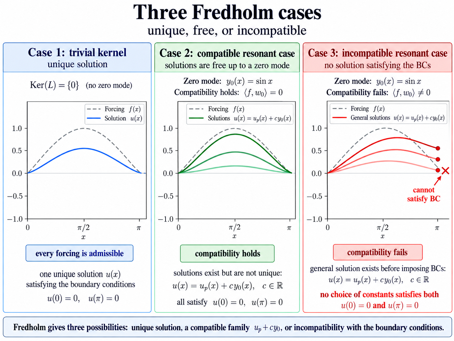
To find the general solution to : \[ \deriv{y}{x}{2} + g_0^2 y = \sin(x). \] We first seek the complementary solution \(y_c\) which solves: \[ \deriv{y_c}{x}{2} + g_0^2 y_c = 0. \] We did this above for the adjoint \(w\) (as this is self adjoint). Thus \[ y_c(x) = A\sin(g_0 x)+ B\cos(g_0 x). \]
We don’t yet apply the boundary conditions, we need the particular solution first.
For the particular solution we seek a solution in the form \(y_p= a_1 \sin(x) + a_2\cos(x)\): which yields
\[ \left(a_1 \left(g_0^2-1\right)-1\right) \sin (x)+a_2 \left(g_0^2-1\right) \cos (x) =0. \tag{3.8}\]
If \(g_0\neq 1\) then we set \(a_2=0\) and \(a_1 = 1/(g_0^2-1)\) and we have a full solution to the problem: \[ y(x) = A\sin(g_0 x)+ B\cos(g_0 x) + \frac{1}{g_0^2-1}\sin(x). \]
This is illustrated in the left panel of Figure 3.1 where it must be that \(A\) and \(B\) are zero (as we showed above). In the middle panel we see the integer (but not \(\pm 1\)) case where \(A\) cannot be fixed.
Confirm this satisfies the boundary conditions if \(g_0\) is an integer greater than \(1\), for any \(A\). If \(g_0\) is not an integer, confirm you need \(A=B=0\), thus uniquely determining the problem.
Thus we have, as Fredholm told us to expect, a solution which is unique if \(g_0\) is not an integer, and non-unique for the compatible integer cases because one homogeneous constant remains free after the boundary conditions are imposed.
But what if \(g_0=1\)? It is clear Equation 3.8 cannot be satisfied. I hope, however, you remember that in such cases we should try a solution in the form: \[ y_p= a_1 x\sin(x) + a_2 x\cos(x), \] as \(\sin(x)\) the right hand side is an eigenfunction of the homogeneous operator, an issue that arises due to the operator having a zero eigenvalue.
Substituting this in we find: \[ 2 a_1 \cos (x)-(2 a_2+1) \sin (x) \] for \(g_0=1\). So we need \(a_1=0\) and \(a_2=-1/2\), so our general solution is: \[ y(x) = A\sin(x)+ B\cos(x) - \frac{1}{2}x\cos(x). \tag{3.9}\]
But wait! Doesn’t this contradict the Fredholm alternative, which told us in this case we cannot have any solution?
Confirm that Equation 3.9 cannot satisfy the boundary conditions \(y(0)=y(\pi)=0\). This is illustrated in the right panel of Figure 3.1. Thus is not a valid solution to the problem.
And you doubted Ivar Fredholm! Shame on you…..
A lot of the failures to be able to solve come not from the fact that there is no general solution to an equation, but that it is not commensurate with the boundary conditions. At the risk of repeating myself the properties of an operator are not fully defined without their boundary conditions.
3.5.1 The coefficient formula revisited.
We recall earlier we found the following general coefficient formula \[ \lambda_k c_k \langle y_k,r(x) w_k\rangle = \langle f,w_k\rangle. \] I asked you to chill on the matter of worrying about the \(\lambda_k=0\) case. Well, now we can address it with Fredholm in mind.
If \(0\) is not an eigenvalue of the adjoint problem, then there is no zero-mode obstruction. If \(0\) is an adjoint eigenvalue, then the corresponding adjoint eigenfunctions lie in \(\ker(L^*)\), and Fredholm tells us that we require \[ \langle f,w\rangle=0 \qquad\text{for every }w\in\ker(L^*). \] In the one-dimensional case this is simply \(\langle f,w_k\rangle=0\) for the zero mode. If the condition fails, we cannot satisfy \(Lu=f\).
So we see Fredholm is intimately related to the ability to construct our series solution
3.6 Extension to higher dimensions
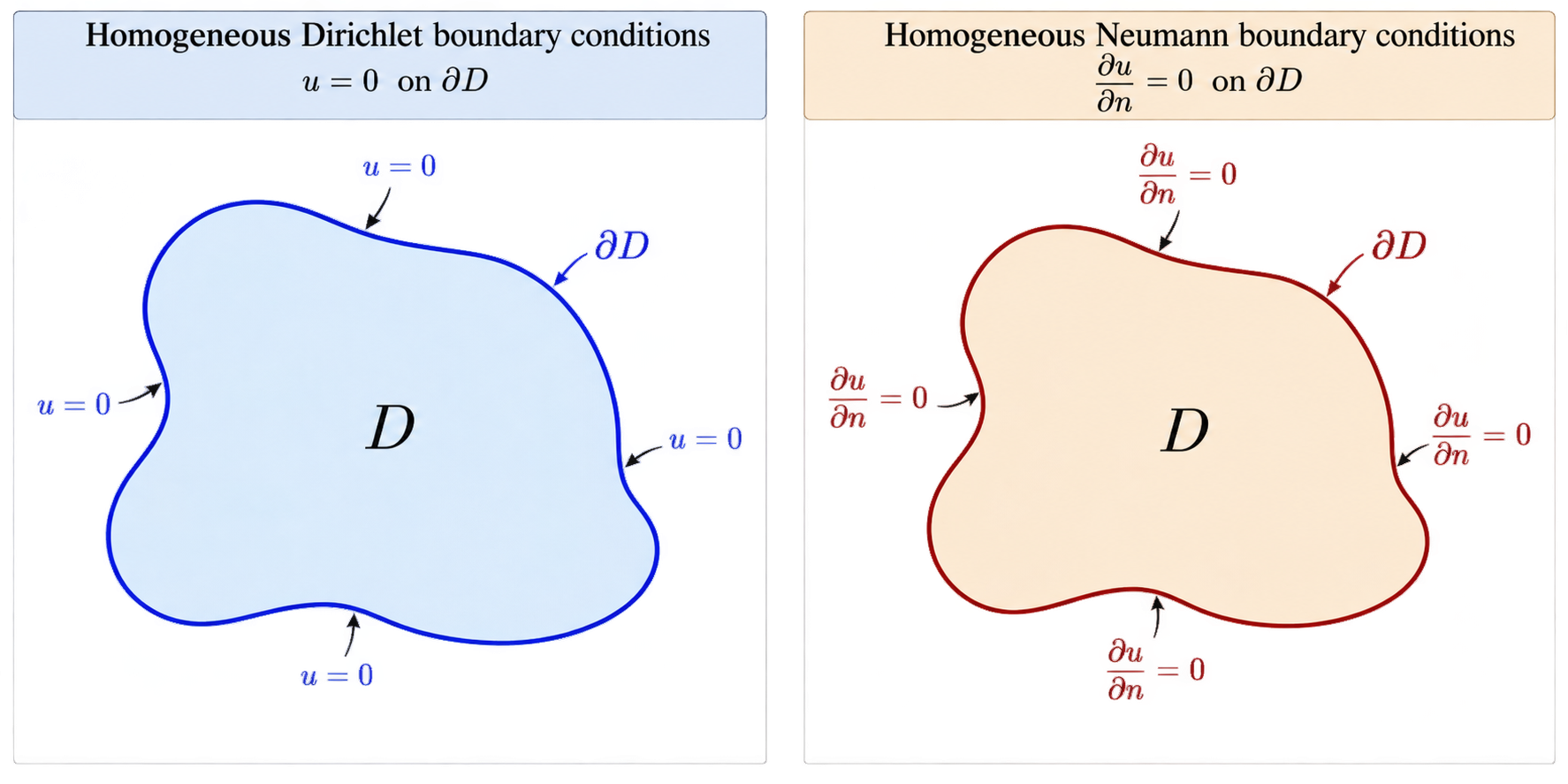
Nothing essential in the ideas above is restricted to one spatial dimension. Let \(\mathcal D\subset\mathbb R^m\) be a spatial domain. For scalar functions on \(\mathcal D\) we use \[ \langle u,v\rangle=\int_{\mathcal D}u(\mathbf x)v(\mathbf x)\,\mathrm{d}V, \] and define the adjoint by the same relation \[ \boxed{\langle Lu,v\rangle=\langle u,L^*v\rangle,} \] with the boundary conditions again forming part of the definition of the operator, the two critical cases are shown in Figure Figure 3.2.
The orthogonality arguments, self-adjointness ideas and Fredholm alternative therefore extend naturally to higher-dimensional operators. What usually becomes harder is not the abstract theory, but finding the eigenfunctions explicitly for a given geometry.
The theory developed in this chapter is therefore not intrinsically one-dimensional. In Chapter 4 we will use it to build eigenfunction expansions for higher-dimensional PDEs; the main practical difficulty is obtaining the spatial eigenfunctions for the chosen geometry and boundary conditions.
We discussed we had completeness for the Sturm Lioville family, crucially we can be confident when everything works out. This actually extends to higher dimensions, but would be too fiddly to state here in its generality. So I have prepared a non-examinable note which has this discussion. It is avaliable in the non-examinable materials section of the Ultra lecture notes tab.
The final challenge, question 14 of the week 8 problem sheet is a length quesiton (much longer than in an exam) which asks you to put this all together, hopefully this will show you it is all at ruly connected theory.
3.7 Summary
The central objects in this chapter were the eigenvalue problem \[ \boxed{Ly=\lambda r(x)y} \] and the inhomogeneous boundary-value problem \[ \boxed{Ly=f.} \]
The main ideas are:
- the boundary conditions are part of the operator problem and affect the adjoint, eigenfunctions and solvability;
- the adjoint \(L^*\) is defined through \(\langle Lu,v\rangle=\langle u,L^*v\rangle\);
- eigenfunctions of \(L\) and \(L^*\) provide the orthogonality needed to obtain general coefficient formulae;
- when \(L=L^*\), the problem is self-adjoint and the eigenfunction theory becomes particularly simple;
- Sturm–Liouville problems give a large and important class of self-adjoint weighted eigenvalue problems;
- the Fredholm alternative tells us when an inhomogeneous BVP \(Ly=f\) can be solved and explains the special role of zero eigenvalues;
- these ideas extend to higher-dimensional operators, although explicit eigenfunctions may become much harder to find.
Chapter 1 showed how functions can be represented in modes, and Chapter 2 showed why PDEs naturally lead to eigenvalue and boundary-value problems. We now have the general mathematical machinery needed to use those modes reliably.
In the next chapter we return to PDEs and apply this theory to problems of the form \[ \boxed{u_t=Lu+h(\mathbf x,t),} \] including different time operators and higher-dimensional spatial domains.