$$ \def\ab{\boldsymbol{a}} \def\bb{\boldsymbol{b}} \def\cb{\boldsymbol{c}} \def\db{\boldsymbol{d}} \def\eb{\boldsymbol{e}} \def\fb{\boldsymbol{f}} \def\gb{\boldsymbol{g}} \def\hb{\boldsymbol{h}} \def\kb{\boldsymbol{k}} \def\nb{\boldsymbol{n}} \def\tb{\boldsymbol{t}} \def\ub{\boldsymbol{u}} \def\vb{\boldsymbol{v}} \def\xb{\boldsymbol{x}} \def\yb{\boldsymbol{y}} \def\Ab{\boldsymbol{A}} \def\Bb{\boldsymbol{B}} \def\Cb{\boldsymbol{C}} \def\Eb{\boldsymbol{E}} \def\Fb{\boldsymbol{F}} \def\Jb{\boldsymbol{J}} \def\Lb{\boldsymbol{L}} \def\Rb{\boldsymbol{R}} \def\Ub{\boldsymbol{U}} \def\xib{\boldsymbol{\xi}} \def\evx{\boldsymbol{e}_x} \def\evy{\boldsymbol{e}_y} \def\evz{\boldsymbol{e}_z} \def\evr{\boldsymbol{e}_r} \def\evt{\boldsymbol{e}_\theta} \def\evp{\boldsymbol{e}_r} \def\evf{\boldsymbol{e}_\phi} \def\evb{\boldsymbol{e}_\parallel} \def\omb{\boldsymbol{\omega}} \def\dA{\;d\Ab} \def\dS{\;d\boldsymbol{S}} \def\dV{\;dV} \def\dl{\mathrm{d}\boldsymbol{l}} \def\rmd{\mathrm{d}} \def\bfzero{\boldsymbol{0}} \def\Rey{\mathrm{Re}} \def\Real{\mathbb{R}} \def\grad{\boldsymbol\nabla} \newcommand{\dds}[2]{\frac{d{#1}}{d{#2}}} \newcommand{\ddy}[2]{\frac{\partial{#1}}{\partial{#2}}} \newcommand{\pder}[3]{\frac{\partial^{#3}{#1}}{\partial{#2}^{#3}}} \newcommand{\deriv}[3]{\frac{d^{#3}{#1}}{d{#2}^{#3}}} \newcommand{\ddt}[1]{\frac{d{#1}}{dt}} \newcommand{\DDt}[1]{\frac{\mathrm{D}{#1}}{\mathrm{D}t}} \newcommand{\been}{\begin{enumerate}} \newcommand{\enen}{\end{enumerate}}\newcommand{\beit}{\begin{itemize}} \newcommand{\enit}{\end{itemize}} \newcommand{\nibf}[1]{\noindent{\bf#1}} \renewcommand{\vec}{\mathbfit} \def\bra{\langle} \def\ket{\rangle} \renewcommand{\S}{{\cal S}} \newcommand{\wo}{w_0} \newcommand{\wid}{\hat{w}} \newcommand{\taus}{\tau_*} \newcommand{\woc}{\wo^{(c)}} \newcommand{\dl}{\mbox{$\Delta L$}} \newcommand{\upd}{\mathrm{d}} \newcommand{\dL}{\mbox{$\Delta L$}} \newcommand{\rs}{\rho_s} $$
2.1 PDEs: the essential setup
A partial differential equation (PDE) is an equation for a function of several independent variables which involves its partial derivatives. For example, the heat/diffusion equation in two spatial dimensions is
\[ \ddy{u}{t}=D\left(\pder{u}{x}{2}+\pder{u}{y}{2}\right), \]
where \(u(x,y,t)\) is the dependent variable, \(x,y,t\) are the independent variables, and \(D>0\) is the diffusion coefficient.
The video shows the characteristic spreading behaviour of diffusion. The same equation can model, for example, heat in a material or the diffusion of a chemical concentration.
For what follows we only need a small amount of terminology:
- the order of a PDE is the order of its highest derivative;
- a PDE is linear if it is linear in the dependent variable \(u\) and its derivatives;
- in this course we will focus mainly on linear PDEs, because linearity allows solutions to be decomposed into independent modes.
A differential operator \(L\) is linear if, for any functions \(u_1,u_2\) and constants \(a,b\),
\[ L(au_1+bu_2)=aLu_1+bLu_2. \]
For example, the heat equation can be written
\[ Lu=0, \qquad L= \ddy{}{t} - D\left( \pder{}{x}{2}+\pder{}{y}{2} \right). \]
Therefore, if \(u_1\) and \(u_2\) are solutions of the homogeneous heat equation,
\[ L(au_1+bu_2) = aLu_1+bLu_2 = 0. \]
So any linear combination of solutions is again a solution. This is the principle of superposition.
More generally, if
\[ Lu_1=f_1, \qquad Lu_2=f_2, \]
then
\[ L(au_1+bu_2)=af_1+bf_2. \]
Thus linearity is not a special feature of the heat equation: it is built into every linear PDE.
For a boundary-value problem we also need the boundary conditions to be linear. If they are homogeneous, a linear combination of solutions satisfies the same boundary conditions. This is exactly what will later allow us to add together many separated solutions to form a Fourier/eigenfunction series.
2.1.1 Boundary and initial conditions
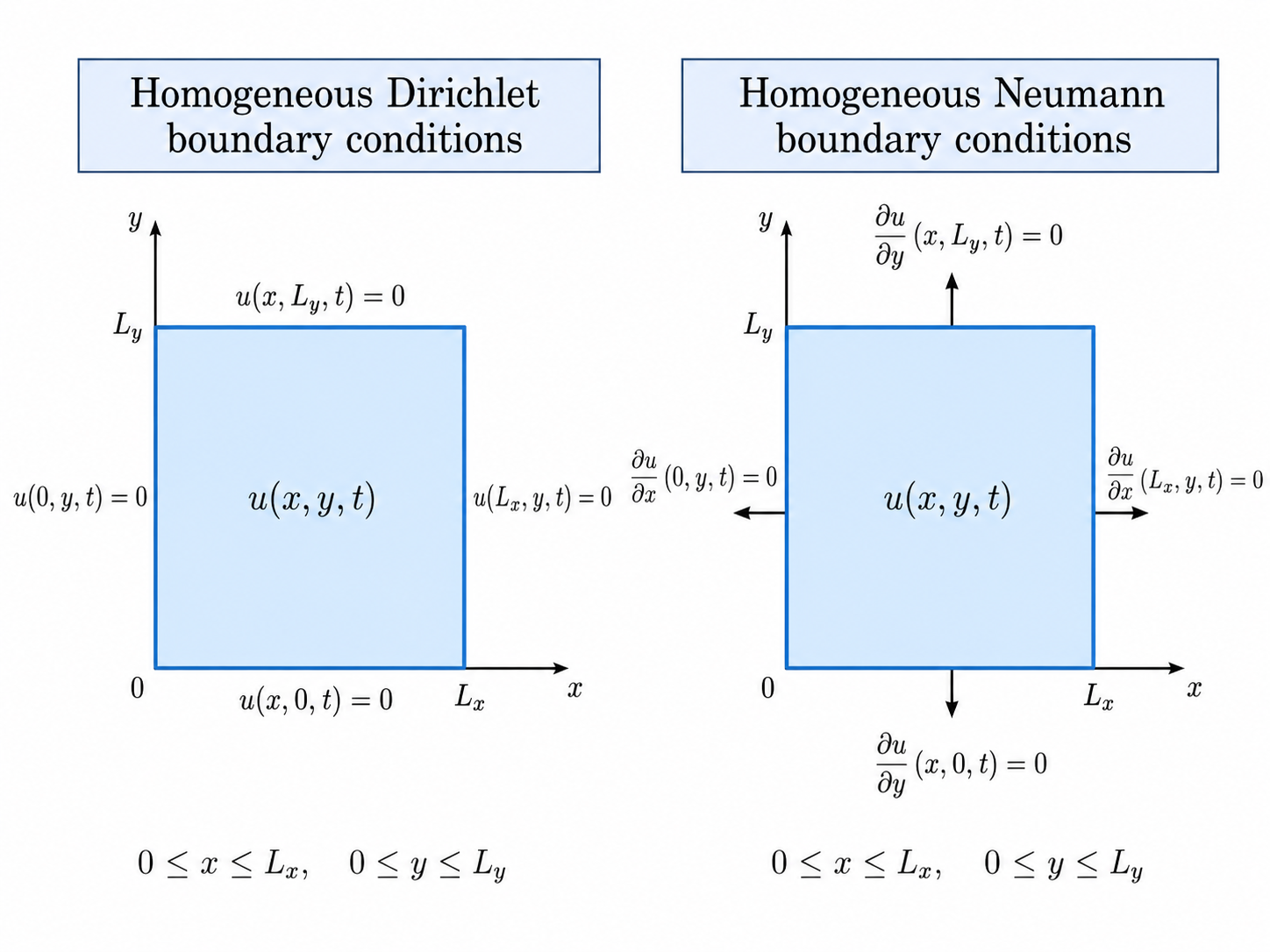
A differential equation is not a complete problem by itself. We must also specify appropriate boundary conditions, and for time-dependent problems usually initial conditions.
For a function \(u(x,y,t)\) on the rectangle \([0,L_x]\times[0,L_y]\), two common homogeneous boundary conditions are:
Dirichlet conditions – specify the value of the function:
\[ u(0,y,t)=u(L_x,y,t)=u(x,0,t)=u(x,L_y,t)=0. \]
Neumann conditions – specify its normal derivative:
\[ \ddy{u}{x}(0,y,t)=\ddy{u}{x}(L_x,y,t)= \ddy{u}{y}(x,0,t)=\ddy{u}{y}(x,L_y,t)=0. \]
To link back to the first half of this course, the compact notation for such boundary conditions on a general domain \(\mathcal{D}\in \mathbb{R}^n\) with boundary \(\partial \mathcal{D}\) are, for (homogeneous) Dirichlet: \[ u({\bf x},t) = 0,\quad \mbox{on all } {\bf x}\in \partial \mathcal{D}, \] and for (homogeneous) Neumann: \[ \nabla u\cdot{\bf n}= 0,\quad \mbox{on all } {\bf x}\in \partial \mathcal{D}, \] where \({\bf n}\) is the (outward) unit normal to \(\partial \mathcal{D}\)
For a time-dependent problem we also prescribe initial data, for example
\[ u(x,y,0)=f(x,y). \] See Figure Figure 2.6
The term homogeneous refers to the boundary data right hand side being equal to zero. Inhomogeneous BCs would be something like: \[ u(0,y,t)=a_1(y),\quad u(L_x,y,t)=a_2(y),\quad u(x,0,t)=a_3(x),\quad u(x,L_y,t)=a_4(x). \] In Chapter 3 we see homogeneous boundary conditions are in some sense fundamental and can be used to construct solutions to problems with inhomogeneous conditions.
Later we will see that changing the boundary conditions can change the permitted modes, the eigenvalues, and ultimately the qualitative behaviour of a solution. We therefore think of a differential equation together with its boundary conditions as the mathematical object to be studied.
Question 1 of the week 7 problem sheet asks you to impose another type of boundary condition, periodicity, on a solution to the heat equation.
Chapter 1 showed us why decomposing functions into simple independent modes is useful. The central question of this chapter is now:
\[ \text{Where do the natural modes of a PDE come from?} \]
For a large class of linear PDEs, the answer begins with separation of variables.
2.2 Separation of variables: from a PDE to eigenvalue problems
We use the heat equation as our main example. Consider
\[ \ddy{u}{t}=D\left(\pder{u}{x}{2}+\pder{u}{y}{2}\right), \]
on \([0,L_x]\times[0,L_y]\), with homogeneous Neumann boundary conditions
\[ \ddy{u}{x}(0,y,t)=\ddy{u}{x}(L_x,y,t)= \ddy{u}{y}(x,0,t)=\ddy{u}{y}(x,L_y,t)=0. \]
We seek a separated solution
\[ u(x,y,t)=X(x)Y(y)T(t). \]
This is the separation ansatz: we assume, for the moment, that the variation in each independent variable can be represented by a separate factor.
2.2.1 Step 1: Separate the variables
Substitution gives
\[ X Y T'=D\left(X''YT+XY''T\right), \]
and dividing by \(DXYT\) gives
\[ \frac{T'}{DT}=\frac{X''}{X}+\frac{Y''}{Y}. \]
The left-hand side depends only on \(t\), while the two terms on the right depend only on \(x\) and \(y\). For the equality to hold for all \(x,y,t\), the separated pieces must be constants. We therefore write
\[ \frac{X''}{X}=-\lambda_x, \qquad \frac{Y''}{Y}=-\lambda_y, \qquad \frac{T'}{DT}=-(\lambda_x+\lambda_y). \]
Thus the PDE has become three ODEs:
\[ X''+\lambda_xX=0, \qquad Y''+\lambda_yY=0, \qquad T'+D(\lambda_x+\lambda_y)T=0. \]
The boundary conditions become
\[ X'(0)=X'(L_x)=0, \qquad Y'(0)=Y'(L_y)=0. \]
Separation of variables has not merely turned one PDE into several ODEs. The spatial equations are ODEs together with boundary conditions:
\[ X''+\lambda_xX=0, \qquad X'(0)=X'(L_x)=0. \]
Non-zero solutions exist only for particular values of \(\lambda_x\). This is an eigenvalue boundary-value problem, i.e. it is in the form: \[ L X = -\lambda_x X \] which has the same structural form as the more familiar matrix eigen-equation \[ A \vec{x} = \lambda \vec{x}. \] The minus sign, is, as we shall see shortly, a convenience to pair positive eigenvalues \(\lambda_x\) with the non-trivial eigenfunctions, i.e. solutions of \(L X = -\lambda_x X\).
2.2.2 Step 2: The boundary conditions select the spatial modes
Consider
\[ X''+\lambda_xX=0, \qquad X'(0)=X'(L_x)=0. \]
Before applying the boundary conditions, let us be explicit about the possible forms of the solution. Try
\[ X=\mathrm{e}^{rx}. \]
Substitution gives the characteristic equation
\[ r^2+\lambda_x=0. \]
The type of solution therefore depends on the roots of this quadratic.
Case 1: \(\lambda_x>0\).
The roots are complex,
\[ r=\pm i\sqrt{\lambda_x}, \]
so the corresponding real form of the solution is
\[ X(x)=A\cos(\sqrt{\lambda_x}x) +B\sin(\sqrt{\lambda_x}x). \]
The first boundary condition gives
\[ X'(0)=B\sqrt{\lambda_x}=0, \]
so \(B=0\). The second gives
\[ X'(L_x)=-A\sqrt{\lambda_x}\sin(\sqrt{\lambda_x}L_x)=0. \]
We are interested in non-trivial solutions, so \(A\neq0\). Hence
\[ \sin(\sqrt{\lambda_x}L_x)=0, \]
which requires
\[ \sqrt{\lambda_x}L_x=m\pi, \qquad m=1,2,3,\ldots \]
Case 2: \(\lambda_x=0\).
The characteristic equation has the repeated root \(r=0\), so
\[ X(x)=A+Bx. \]
The Neumann boundary conditions give \(B=0\), leaving the non-zero constant solution.
Case 3: \(\lambda_x<0\).
Write
\[ \lambda_x=-\mu^2, \qquad \mu>0. \]
The characteristic equation becomes
\[ r^2-\mu^2=0, \]
with two real roots
\[ r=\pm\mu. \]
Hence
\[ X(x)=A \mathrm{e}^{\mu x}+B\mathrm{e}^{-\mu x}. \]
These exponential solutions cannot satisfy both Neumann boundary conditions non-trivially.
Starting from
\[ X=A\mathrm{e}^{\mu x}+B\mathrm{e}^{-\mu x}, \]
use \(X'(0)=X'(L_x)=0\) to show that \(A=B=0\) is the only possibility.
The characteristic equation is particularly simple here, but it is worth keeping this route in mind. For a more general constant-coefficient equation
\[ aX''+bX'+cX=0, \]
we obtain
\[ ar^2+br+c=0. \]
The discriminant \(b^2-4ac\) tells us whether the roots are two real roots, one repeated real root, or a complex-conjugate pair. In later examples containing first-derivative terms, this is the reliable way to decide which form of the solution to use.
Questions 2-4 of the week 7 problem sheet give you practice at solving this kind of eigen-equation (with constant coefficients), using the method which follows to impose boundary conditions. Something like this is certain to turn up on the exam, AND we will need it for all the following sections. So make sure you are on top of it.
Combining the admissible cases gives
\[ \lambda_{x,m}=\left(\frac{m\pi}{L_x}\right)^2, \qquad X_m(x)=\cos\left(\frac{m\pi x}{L_x}\right), \qquad m=0,1,2,\ldots \]
The \(Y\) problem is identical, giving
\[ \lambda_{y,n}=\left(\frac{n\pi}{L_y}\right)^2, \qquad Y_n(y)=\cos\left(\frac{n\pi y}{L_y}\right). \]
Hence the permitted spatial modes are
\[ \Phi_{mn}(x,y)= X(x)Y(y)= \cos\left(\frac{m\pi x}{L_x}\right) \cos\left(\frac{n\pi y}{L_y}\right), \]
with spatial eigenvalues
\[ \lambda_{mn}= \left(\frac{m\pi}{L_x}\right)^2+ \left(\frac{n\pi}{L_y}\right)^2. \]
The cosine modes have therefore not been chosen because we happened to know a Fourier series. They have been selected by the spatial differential equation and the boundary conditions.
Different boundary conditions would select different modes. For example, homogeneous Dirichlet conditions on a rectangular domain select sine modes instead.
Questions 4–6 of problem sheet 1 give further practice with spatial separation and boundary conditions.
2.2.3 Step 3: The PDE determines how each mode evolves
For each spatial mode \((m,n)\), the time factor satisfies
\[ T_{mn}'+D\lambda_{mn}T_{mn}=0, \]
so
\[ T_{mn}(t)=a_{mn}\mathrm{e}^{-D\lambda_{mn}t}. \]
Each separated solution we have constructed satisfies the same linear homogeneous heat equation and the same homogeneous boundary conditions. Therefore the superposition principle above tells us that linear combinations of them are also solutions. Passing to the corresponding convergent eigenfunction/Fourier expansion gives the modal solution
\[ u(x,y,t)=\sum_{m=0}^{\infty}\sum_{n=0}^{\infty} a_{mn}\mathrm{e}^{-D\lambda_{mn}t}\Phi_{mn}(x,y). \tag{2.1}\]
The initial condition now determines the amplitudes \(a_{mn}\). If
\[ u(x,y,0)=f(x,y), \]
then at \(t=0\) we require
\[ f(x,y)=\sum_{m=0}^{\infty}\sum_{n=0}^{\infty}a_{mn}\Phi_{mn}(x,y). \]
This is exactly the type of expansion considered in Chapter 1, so orthogonality gives the coefficient grab
\[ a_{mn}=\frac{\langle f,\Phi_{mn}\rangle} {\langle\Phi_{mn},\Phi_{mn}\rangle}. \]
The PDE and boundary conditions tell us which modes are allowed and how each one evolves; the initial condition tells us how much of each mode is present.
Suppose the initial temperature is
\[ f(x,y)=3 +2\cos\left(\frac{\pi x}{L_x}\right) \cos\left(\frac{2\pi y}{L_y}\right) -\cos\left(\frac{3\pi x}{L_x}\right). \]
In terms of the spatial eigenmodes this is simply
\[ f=3\Phi_{00}+2\Phi_{12}-\Phi_{30}. \]
Equivalently, the coefficient-grab formula from Chapter 1 gives
\[ a_{00}=3,\qquad a_{12}=2,\qquad a_{30}=-1, \]
with all other coefficients zero. Therefore
\[ \begin{aligned} u(x,y,t)={}&3\Phi_{00} +2\mathrm{e}^{-D\lambda_{12}t}\Phi_{12} -\mathrm{e}^{-D\lambda_{30}t}\Phi_{30}\\ ={}&3 +2\mathrm{e}^{-D\left[(\pi/L_x)^2+(2\pi/L_y)^2\right]t} \cos\left(\frac{\pi x}{L_x}\right) \cos\left(\frac{2\pi y}{L_y}\right)\\ &-\mathrm{e}^{-D(3\pi/L_x)^2t} \cos\left(\frac{3\pi x}{L_x}\right). \end{aligned} \]
So the initial condition fixes the modal amplitudes, while the heat equation subsequently makes each non-constant mode decay at its own rate. The constant mode remains.
In many practical uses of this method the initial conditions are not important and we would have been happy to stop at Equation 2.1 (e.g. stability analysis which is crucial in many third year topics). As an example of why, we note in this case whatever the values of \(n\) all modes (except \((n,m)=(0,0)\)) decay to \(0\) as \(t\rightarrow \infty\)
Questions 5 and 6 of the week 7 problem sheet gives practice with the full separation-of-variables method. 5 shows you how to use it in different coordinate systems, 6 how to transform equations so the method works.
2.3 Same spatial eigenproblem, different time evolution
The spatial eigenvalue problem and the temporal equation play different roles. For the heat equation we have just found
\[ T_{mn}'+D\lambda_{mn}T_{mn}=0, \]
so
\[ T_{mn}(t)=a_{mn}\mathrm{e}^{-D\lambda_{mn}t}. \]
Higher spatial modes have larger \(\lambda_{mn}\) and therefore decay more rapidly. The constant mode \(\lambda_{00}=0\) does not decay.
| 1D heat-equation evolution | 2D heat-equation evolution |
The heat equation therefore progressively removes small-scale structure. This behaviour matches the other name given to the equation: the diffusion equation. If the zero mode is permitted, the long-time state tends towards a spatially uniform value.
Now consider the wave equation with the same spatial operator and the same Neumann boundary conditions,
\[ \pder{u}{t}{2}=c^2\left(\pder{u}{x}{2} + \pder{u}{y}{2} \right). \tag{2.2}\]
The entire spatial calculation above is unchanged: the allowed \(\Phi_{mn}\) and \(\lambda_{mn}\) are exactly the same. The only difference is the temporal ODE,
\[ T_{mn}''+c^2\lambda_{mn}T_{mn}=0, \]
Work through the steps we used in section 2.2 to solve the heat equation applied to this wave equation Equation 2.2 in order to confirm this is indeed the only difference.
so, for \(\lambda_{mn}>0\),
\[ T_{mn}(t)=A_{mn}\cos(c\sqrt{\lambda_{mn}}t) +B_{mn}\sin(c\sqrt{\lambda_{mn}}t). \]
Thus the same spatial modes now oscillate rather than decay (and the initial conditions would very much matter!). A full wave problem requires two initial conditions, for example \(u(x,y,0)\) and \(u_t(x,y,0)\); projecting both onto the same spatial modes determines the constants \(A_{mn}\) and \(B_{mn}\).
2.3.1 Heat versus wave evolution
The videos compare heat-equation and wave-equation solutions starting from similar initial data. The heat equation damps the higher modes and smooths the solution, while the wave equation retains oscillatory modal behaviour.
The heat equation is the prototype parabolic PDE, while the wave equation is the prototype hyperbolic PDE. Their very different temporal mode equations already give us a first indication of their different qualitative behaviour (one aspect of which is that parabolic equations tend to smooth/simplify solutions whilst hyperbolic equations can maintain the initial complexity).
If you are interested in having this distinction made much more precise I would advise you take the third year Partial Differential Equations course.
2.3.2 Modes can also grow
The heat equation gives decay and the wave equation gives oscillation, but individual modes can also grow. In many linear or linearised systems, after expanding in spatial eigenmodes, a modal amplitude satisfies an equation of the form
\[ T_{mn}'=\sigma_{mn}T_{mn}. \]
The sign of the growth rate \(\sigma_{mn}\) determines the behaviour of that particular mode:
\[ \sigma_{mn}<0 \Rightarrow \text{decay},\qquad \sigma_{mn}=0 \Rightarrow \text{neutral},\qquad \sigma_{mn}>0 \Rightarrow \text{growth}. \]
This makes the idea from Chapter 1 very concrete: different independent spatial components can have genuinely different dynamics.
Question 10 of the week 7 problem sheet has a nice physically motivated bacterial flow problem for which you can have both mode growth and decay (dependent on system parameters). Its longer than an exam question, but parts could very well be the type of question which turns up on an exam.
A classic example occurs in coupled reaction–diffusion systems. For suitable parameters, most modes decay but a small range has positive growth rates. This is the basis of the Turing mechanism for pattern formation: selected spatial modes are amplified and, in the full nonlinear system, are later stabilised rather than growing without bound.
The video shows a reaction–diffusion system developing an ordered spotted pattern. The important point here is not the detailed model, but that the PDE can select particular spatial modes and determine whether they decay, oscillate or grow.
2.4 Geometry changes the spatial eigenvalue problem
The rectangular examples might suggest that sine and cosine functions are somehow fundamental to linear PDEs. They are not. They arise because of the combination of the differential operator, the geometry, and the boundary conditions.
A classic example is the heat equation on a disc.
2.4.1 Bessel functions and the heat equation on a disc
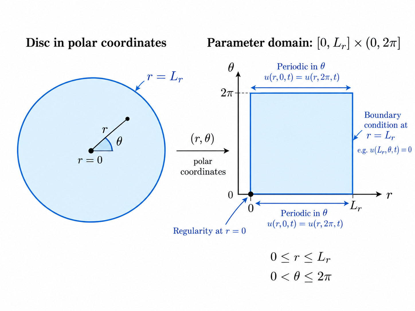
Consider
\[ \ddy{u}{t}=D\nabla^2u, \qquad (r,\theta)\in[0,L_r]\times(0,2\pi], \] where: \[ \nabla^2=\nabla\cdot\nabla \]
The coordinate free definition of the Laplacian is: \[ \nabla^2=\nabla\cdot\nabla \] another common notation is \(\triangle =\nabla\cdot\nabla\) (more common in mathematical analysis). In Cartesian coordinates: \[ \nabla^2u = \pder{u}{x}{2} + \pder{u}{y}{2}. \] so \[ \ddy{u}{t}=D\nabla^2u \] is the heat equation in a general coordinate system.
We solve this problem subject to homogeneous Dirichlet boundary conditions: \[ u(L_r,\theta,t)=0, \] and periodicity in \(\theta\): \(u(r,\theta,t)= u(r,\theta+2\pi,t)\). See Figure Figure 2.2 for an illustration of the domain and BCs.
We seek a separated solution
\[ u(r,\theta,t)=R(r)P(\theta)T(t). \]
Separating time from space gives
\[ \frac{T'}{DT}=-\lambda, \qquad \nabla^2(RP)+\lambda RP=0. \]
In polar coordinates,
\[ \nabla^2y= \frac{1}{r}\ddy{}{r}\left(r\ddy{y}{r}\right) +\frac{1}{r^2}\pder{y}{\theta}{2}. \]
Substituting \(y=R(r)P(\theta)\) and multiplying by \(r^2/(RP)\) gives
\[ \frac{r}{R}\dds{}{r}\left(r\dds{R}{r}\right)+\lambda r^2 =-\frac{P''}{P}. \]
Again the two sides depend on independent variables, so both must equal a constant. Write
\[ -\frac{P''}{P}=\lambda_\theta. \]
The angular problem is therefore
\[ P''+\lambda_\theta P=0, \]
with periodic boundary conditions \(P(\theta)= P(\theta+2\pi)\). These require
\[ \lambda_\theta=n^2, \qquad P_n(\theta)=A\cos(n\theta)+B\sin(n\theta), \qquad n=0,1,2,\ldots \]
The radial equation becomes
\[ r^2R''+rR'+(\lambda r^2-n^2)R=0. \]
This is Bessel’s equation.
Bessel’s equation can be solved by the Frobenius power-series method encountered in Calculus I. We will not repeat that calculation here. For our purposes the important point is what its solutions do and how the boundary conditions select them.
The solution which remains finite at the origin is the Bessel function of the first kind,
\[ R(r)=J_n(\sqrt{\lambda}\,r). \]
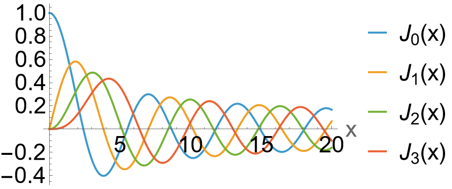
The outer Dirichlet condition requires
\[ R(L_r)=0 \quad\Rightarrow\quad J_n(\sqrt{\lambda}L_r)=0. \]
Let \(j_{n,k}\) denote the \(k\)th positive zero of \(J_n\). Then the permitted eigenvalues are
\[ \lambda_{n,k}=\left(\frac{j_{n,k}}{L_r}\right)^2. \]
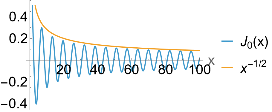
The corresponding spatial eigenmodes are
\[ \Phi^{(c)}_{n,k}(r,\theta)= J_n\left(\frac{j_{n,k}r}{L_r}\right)\cos(n\theta), \]
and
\[ \Phi^{(s)}_{n,k}(r,\theta)= J_n\left(\frac{j_{n,k}r}{L_r}\right)\sin(n\theta). \]
For fixed \(n\), the radial Bessel functions are orthogonal with the polar-coordinate weight \(r\):
\[ \left\langle J_n\left(\frac{j_{n,k}r}{L_r}\right), \,rJ_n\left(\frac{j_{n,\ell}r}{L_r}\right) \right\rangle=0, \qquad k\neq\ell. \]
This is exactly the kind of weighted orthogonality introduced in Chapter 1.
“Fun” fact: G. N. Watson’s classic Treatise on the Theory of Bessel Functions runs to more than 800 pages. This is what folk did to pass their spare time before the internet. We are going to use rather less of it.
2.4.2 The full modal solution
The temporal equation is
\[ T_{n,k}'+D\lambda_{n,k}T_{n,k}=0, \]
so
\[ T_{n,k}(t)=C_{n,k}\mathrm{e}^{-D\lambda_{n,k}t}. \]
Hence the solution is built from Fourier–Bessel modes:
\[ u(r,\theta,t) ={}\sum_{n=0}^{\infty}\sum_{k=1}^{\infty} \mathrm{e}^{-D\lambda_{n,k}t} J_n\left(\frac{j_{n,k}r}{L_r}\right)\left[ A_{n,k}\cos(n\theta)+B_{n,k}\sin(n\theta) \right]. \]
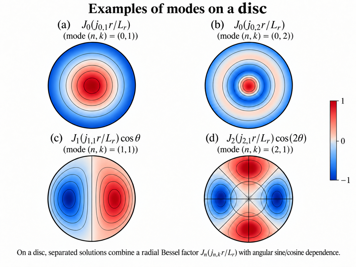
Some examples are shown in Figure 2.5
At \(t=0\), an initial condition \(f(r,\theta)\) is expanded in the same spatial modes. Chapter 1 means that we no longer need to work through the coefficient integrals from scratch. If \(\Phi_{n,k}\) denotes one of the spatial modes, then schematically
\[ A_{n,k}= \frac{\langle f,r\Phi_{n,k}\rangle} {\langle\Phi_{n,k},r\Phi_{n,k}\rangle}. \]
The weight \(r\) appears explicitly because the polar area element is \(r\,\mathrm{d}r\,\mathrm{d}\theta\). For reference this is written concretely as: \[ A_{n,k}= \frac{\int_{0}^{2\pi}\int_{0}^{L_r} f J_n\left(\frac{j_{n,k}r}{L_r}\right)\cos(n\theta)r\, \mathrm{d}r\, \mathrm{d}\theta} {\int_{0}^{2\pi}\int_{0}^{L_r} J_n^2\left(\frac{j_{n,k}r}{L_r}\right)\cos^2(n\theta)r\, \mathrm{d}r\, \mathrm{d}\theta} \]
On a rectangle, the spatial boundary-value problem selected sine and cosine modes. On a disc, it selected Fourier–Bessel modes. The basic mechanism is the same:
\[ \text{operator + domain geometry + boundary conditions} \longrightarrow \text{eigenvalues and eigenfunctions}. \]
Problem 9 of problem sheet 1 gives practice with Bessel orthogonality, while problem 10 considers a spherical geometry involving spherical Bessel functions and Legendre polynomials.
Questions 7 and 8 of the week 7 problem sheet cover aspects of separation of variables in non-Euclidean (non-rectangular) domains.
Question 11 of the week 7 problem sheet considers a more complex equation (advective) and boundary condition, and shows we can reuse much of our analysis via a transformation.
2.5 Eigenvalue problems are more fundamental than separation of variables
Separation of variables is a very useful way of finding eigenfunctions, but it is not the fundamental method.
The more important idea is that, once we have found a suitable family of eigenfunctions for a differential operator, and its boundary conditions, as we did in sections 2.2–2.4 above, the results of Chapter 1 allow us to use those eigenfunctions as a basis for representing general functions.
A simple example to illustrate this utility and where where separation of variables fails is the forced Poisson problem on the square
\[ -\nabla^2u=f(x,y),\quad 0<x<\pi,\qquad 0<y<\pi, \]
with homogeneous Dirichlet boundary conditions,
\[ u=0\quad\text{on the boundary}. \]
2.5.1 Why separation of variables no longer works directly
Suppose we try to solve the forced problem using a single separated solution
\[ u(x,y)=X(x)Y(y). \]
Substitution into
\[ -\nabla^2u=f(x,y) \]
gives
\[ -X''(x)Y(y)-X(x)Y''(y)=f(x,y). \]
Dividing by \(X(x)Y(y)\) gives
\[ -\frac{X''(x)}{X(x)} -\frac{Y''(y)}{Y(y)} = \frac{f(x,y)}{X(x)Y(y)}. \]
The left-hand side necessarily has the special separated form
\[ F(x)+G(y), \]
but for a general forcing \(f(x,y)\) the right-hand side has no reason to have this form.
So, in general,
\[ u(x,y)=X(x)Y(y) \]
cannot solve the forced problem.
This is where the results of Chapter 1 become crucial.
2.5.2 Chapter 1 already tells us how to deal with the forcing
In Chapter 1 we saw that, given a suitable complete orthogonal basis \(\{\phi_{\vec{k}}\}\), a general function can be represented as
\[ f=\sum_{\vec{k}}f_{\vec{k}}\phi_{\vec{k}}. \] That is exactly what we need here.
The idea is to use functions \(\phi_{mn}\) obtained from the corresponding homogeneous eigenvalue problem. Since we are solving: \[ -\nabla^2u=f(x,y), \qquad u=0\quad\text{on the boundary}. \] The corresponding eigenfunction problem is \[ -\nabla^2\phi=\lambda\phi, \qquad \phi=0\quad\text{on the boundary}. \]
Separation of variables gives the familiar eigenfunctions (hence the basis is separable!): \[ \phi_{mn}(x,y)=\sin(mx)\sin(ny), \qquad \lambda_{mn}=m^2+n^2, \qquad m,n=1,2,\ldots \] We therefore expand the forcing as
\[ f(x,y)= \sum_{m=1}^{\infty} \sum_{n=1}^{\infty} f_{mn}\phi_{mn}(x,y), \]
where, using the coefficient-grab formula from Chapter 1,
\[ f_{mn} = \frac{\langle f,\phi_{mn}\rangle} {\langle\phi_{mn},\phi_{mn}\rangle}. \]
So Chapter 1 has already told us how to represent the right-hand side of the equation.
We now seek the unknown function in exactly the same basis,
\[ u(x,y)= \sum_{m=1}^{\infty} \sum_{n=1}^{\infty} a_{mn}\phi_{mn}(x,y). \]
The key advantage of using eigenfunctions is that the differential operator acts on each basis function in an exceptionally simple way:
\[ -\nabla^2\phi_{mn} = \lambda_{mn}\phi_{mn}. \]
Therefore
\[ \begin{aligned} -\nabla^2u &= -\nabla^2 \left( \sum_{m,n}a_{mn}\phi_{mn} \right)\\ &= \sum_{m,n}a_{mn} \left(-\nabla^2\phi_{mn}\right)\\ &= \sum_{m,n}\lambda_{mn}a_{mn}\phi_{mn}. \end{aligned} \]
But
\[ -\nabla^2u=f, \]
and Chapter 1 gives
\[ f= \sum_{m,n}f_{mn}\phi_{mn}. \]
Hence
\[ \sum_{m,n}\lambda_{mn}a_{mn}\phi_{mn} = \sum_{m,n}f_{mn}\phi_{mn}. \]
Since the modes/eigenfunctions \(\phi_{mn}\) are independent,
\[ \lambda_{mn}a_{mn}=f_{mn} \]
for every \((m,n)\), and therefore
\[ a_{mn} = \frac{f_{mn}}{\lambda_{mn}} = \frac{f_{mn}}{m^2+n^2}. \]
Chapter 1 showed us how to represent a function as a sum of independent modes:
\[ f=\sum_n f_n\phi_n. \]
We are now taking the next step.
We want to solve equations of the form
\[ Lu=f, \]
where a linear operator acts on one function to produce another function.
If we choose the basis functions to be eigenfunctions of \(L\),
\[ L\phi_n=\lambda_n\phi_n, \]
then
\[ u=\sum_n a_n\phi_n \]
implies
\[ Lu=\sum_n\lambda_n a_n\phi_n. \]
Comparing with
\[ f=\sum_n f_n\phi_n \]
gives
\[ \lambda_n a_n=f_n. \]
So the differential equation between functions becomes a set of simple algebraic equations between modal coefficients.
This is the key step beyond Chapter 1, and it is the central reason that eigenvalue problems are so useful.
2.6 What about nonlinear PDEs?
The superposition principle does not hold for nonlinear PDEs, so the simple linear theory cannot be transferred unchanged. Nevertheless, the same mode ideas remain extremely useful.
A common nonlinear extension of the heat equation is a reaction–diffusion equation such as
\[ \ddy{u}{t}=D\nabla^2u+f(u), \] where \(f(u)\) is a non linear function. More commonly in realistic models there are coupled system of such equations :
\[\begin{align} &\ddy{u_1}{t}=D_1\nabla^2u_1+f_1(u_1,u_2),\\ &\ddy{u_2}{t}=D_2\nabla^2u_2+f_2(u_1,u_2) \end{align}\]
The diffusion operator and the boundary conditions still provide a natural spatial eigenbasis. We can therefore represent the solution schematically as
\[ u(\mathbf{x},t)=\sum_n a_n(t)\phi_n(\mathbf{x}), \]
where the \(\phi_n\) are eigenfunctions of the corresponding linear spatial operator on that geometry.
The crucial difference from the linear case is that the nonlinear term \(f(u)\) generally couples the modal amplitudes together. Instead of obtaining one independent ODE for each coefficient, we obtain a coupled system for the \(a_n(t)\). The basis is still useful: it turns a complicated spatial problem into equations describing how the amplitudes of spatial patterns interact.
This is the basic idea behind many spectral methods for nonlinear PDEs. Often one uses the eigenfunctions of the dominant linear spatial operator: Fourier modes on periodic or rectangular geometries, for example, or Bessel modes on a disc. Other spectral bases, such as Chebyshev polynomials on finite intervals, are also widely used because they can represent smooth functions very efficiently.
The reaction–diffusion pattern shown above is a good example: linear eigenvalue analysis identifies which spatial modes initially grow, while the nonlinear terms determine how those growing modes interact and eventually saturate.
For more visual examples of linear and nonlinear PDE behaviour, we will use VisualPDE in class. The point here is not to develop nonlinear PDE theory, but to see why the linear eigenmodes studied in this course remain useful even when the full equation is nonlinear.
2.7 Why this leads us to eigenvalue and boundary-value problems
The examples in this chapter have progressively shifted the emphasis away from separation of variables itself.
- On the rectangle, separation exposed the sine and cosine eigenfunctions selected by the operator and boundary conditions.
- On the disc, the same process produced Bessel eigenfunctions instead.
- In the forced Poisson problem, the eigenfunctions of the homogeneous problem solved an inhomogeneous problem which need not itself separate.
- For nonlinear PDEs, the same spatial bases remain useful, but the nonlinear terms couple their amplitudes together.
The common mathematical object is therefore the eigenvalue boundary-value problem. We write it abstractly as
\[ \boxed{Ly=\lambda r(x)y,} \]
subject to specified boundary conditions.
The sign of \(\lambda\) is a convention. What matters is that non-trivial solutions occur only for particular values of \(\lambda\), and that the corresponding eigenfunctions provide the natural modes with which we analyse more general differential equations.
The forced example also introduced a second object which will become increasingly important:
\[ \boxed{Lu=f,} \]
again subject to boundary conditions. Understanding when such an inhomogeneous boundary-value problem can be solved, and how its solution can be represented using eigenfunctions, requires more general theory.
By this point you should understand the main ideas behind using mode decompositions to study partial differential equations:
A PDE must be considered together with its domain, boundary conditions and, where appropriate, initial conditions.
Separation of variables can reduce a PDE to ordinary differential equations. Crucially, the spatial equations are often boundary-value eigenvalue problems.
The permitted spatial modes are determined by the combination
\[ \boxed{ \text{operator + domain geometry + boundary conditions} \longrightarrow \text{eigenvalues and eigenfunctions}. } \]
On a rectangle these may be sine and cosine modes; on a disc they may involve Bessel functions.
Once the spatial modes are known, the PDE determines how the amplitude of each mode evolves. Different PDEs can have the same spatial eigenfunctions but very different modal dynamics: modes may decay, oscillate or grow.
The results of Chapter 1 then become directly useful.when the eigenfunctions form a suitable complete basis, a general initial condition or forcing can be expanded in the eigenfunctions,
\[ f=\sum_n f_n\phi_n, \]
and the differential operator acts particularly simply on this basis because
\[ L\phi_n=\lambda_n\phi_n. \]
This allows us to go beyond simply representing functions. We can use mode decompositions to solve equations between functions,
\[ Lu=f. \]
If
\[ u=\sum_n a_n\phi_n, \qquad f=\sum_n f_n\phi_n, \]
then, in the simplest case,
\[ Lu=f \qquad\Longrightarrow\qquad \lambda_n a_n=f_n. \]
Separation of variables is therefore a useful way of finding eigenfunctions, but it is not the general theory. Forcing terms, complicated domains or boundary conditions may prevent a problem from being solved by a single product such as \(X(x)Y(y)\), while an eigenfunction expansion may still be useful.
The central progression from Chapters 1 and 2 is therefore
\[ \boxed{ \begin{array}{c} \text{represent functions using modes}\\[2mm] \Downarrow\\[2mm] \text{find modes adapted to a differential operator and its boundary conditions}\\[2mm] \Downarrow\\[2mm] \text{use those modes to solve equations involving the operator.} \end{array} } \]
This leaves us with the general mathematical questions behind the method. Given boundary-value problems of the form
\[ L\phi=\lambda r(x)\phi \]
and
\[ Lu=f, \]
when do suitable eigenfunctions exist? When are they orthogonal and complete? How do we calculate expansion coefficients in the general case? How do the boundary conditions enter the theory? When does the inhomogeneous problem \(Lu=f\) have a solution? And what changes when \(L\) does not possess the symmetry property we will call self-adjointness?
These are the questions developed in the next chapter.