1  Probability

1.1 Introduction to Probability

1.1.1 What is probability?

Probability is how we quantify uncertainty; it is the extent to which an event is likely to occur. We use it to study events whose outcomes we do not (yet) know, whether this is because they have not happened yet, or because we have not yet observed them.

We quantify this uncertainty by assigning each event a number between 0 and 1. The higher the probability of an event, the more likely it is to occur.

Historically, the early theory of probability was developed in the context of gambling. In the seventeenth century, Blaise Pascal, Pierre de Fermat, and the Chevalier de Méré were interested in questions like “If I roll a six-sided die four times, how likely am I to get at least one six?” and “if I roll a pair of dice twenty-four times, how likely am I to get at least one pair of sixes?” Many of the examples we’ll see in this course still use situations like rolling dice, drawing cards, or sticking your hand into a bag filled with differently-coloured tokens.

Nowadays, probability theory helps us to understand how the world around us works, such as in the study of genetics and quantum mechanics; to model complex systems, such as population growth and financial markets, and to analyse data, via the theory of statistics.

We’ll see a bit of statistical theory at the end of this chapter, but will mostly stay on the probabilistic side of that line.

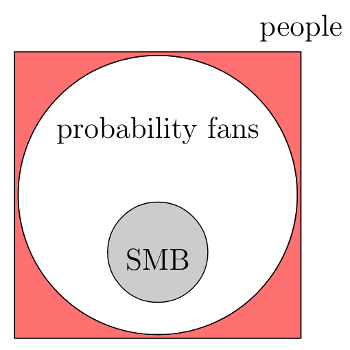
1.1.2 Events

Definition

We use probability theory to describe scenarios in which we don’t know what the outcome will be. We call these scenarios experiments or trials.

The set of all possible outcomes of an experiment is its sample space, \(S\). Subsets of \(S\) are called events, and may contain several different outcomes.

Examples

In the experiment in which we roll a single six-sided die, we have:

• The sample space is \(S = \{ 1,2,3,4,5,6\}\)

• An example of a possible outcome is 5 (or “we roll a five”)

• An example of an event is \(A = \{2,4,6\}\) (or “we roll an even number”).

Because events are subsets of the sample space, we can treat them as sets.

1.1.2.1 Set operations

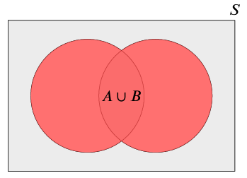
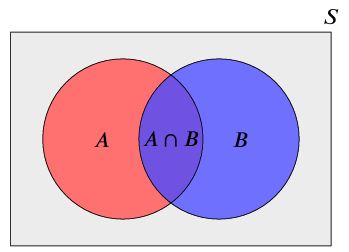
There are three basic operations we can use to combine and manipulate sets.

Definition

If \(A\) and \(B\) are events, then

• The event not \(A\), which we write \(A^c\) (the \(c\) is for complement), is the set of all outcomes in \(S\) which are not in \(A\).

• The event \(A\) or \(B\), which we write \(A \cup B\) and call the union of \(A\) and \(B\), is the set of all outcomes which are in at least one of \(A\) and \(B\).

• The event \(A\) and \(B\), which we write \(A \cap B\) and call the intersection of \(A\) and \(B\), is the set of all outcomes which are in both \(A\) and \(B\).

(a)

(b)

(c)

(d)

Figure 1.1: Pictures illustrating: (a) \(A\); (b) \(A \cup B\); (c) \(A \cap B\); and (d) \(A \setminus B\).

1.1.2.2 Working with events

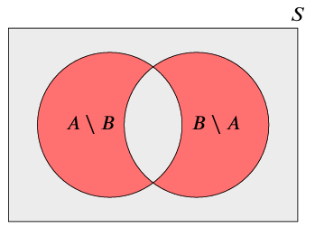
When we want to consider all the outcomes in an event \(A\) which are not in \(B\), we write \(A \cap B^c = A \setminus B\).

We say that two events are disjoint (or incompatible, or mutually exclusive) if they cannot occur at the same time; in other words, if \(A\) and \(B\) are disjoint, then \(A \cap B\) contains no outcomes.

We write \(A \cap B = \emptyset\), and we call \(\emptyset\) the empty set.

If every outcome in an event \(A\) is also in an event \(B\), we say that \(A\) is a subset of \(B\), and we write \(A \subseteq B\).

Examples

For example, since all Single Maths students are fans of probability, \[\begin{aligned} \{ \text{Single Maths students} \} \subseteq \{ \text{Fans of probability} \}. \end{aligned}\]

We can depict this in a diagram: see Figure 1.2 below.

Figure 1.2: Notice that the circle of “probability fans“ takes up quite a lot of the sample space.

The following set of basic rules will be helpful when working with events.

Commutativity: \[ A\cup B = B\cup A, \quad A\cap B= B\cap A\] Associativity: \[(A\cup B)\cup C = A\cup( B\cup C), \quad ( A\cap B)\cap C= A\cap(B\cap C)\] Distributivity: \[(A\cap B)\cup C = (A\cup C)\cap( B\cup C), \quad (A\cup B)\cap C=(A\cap C)\cup( B\cap C)\] De Morgan’s laws: \[(A\cup B)^c = {A}^c\cap{B}^c, \quad (A\cap B)^c ={A}^c\cup{B}^c \]

Example

For example, if \(A = \{\text{Dinner is on time} \}\) and \(B = \{ \text{Dinner is delicious} \}\), then \[\begin{aligned} (A \cap B)^c = \{ \text{Dinner is either late or disappointing} \}, \end{aligned}\] and \[\begin{aligned} (A \cup B)^c = \{ \text{Dinner is \emph{both} late \emph{and} disappointing} \}. \end{aligned}\]

1.1.3 Axioms of Probability

Once we have decided what our experiment (and hence our sample space) should be, we assign a probability to each event \(A \subseteq S\). This probability is a number, which we write \(\mathbb{P}(A)\).

Remember that \(A\) is an event, which is a set, and that \(\mathbb{P}(A)\) is a probability, which is a number. It makes sense to take the union of sets, or to add numbers together - but not the other way around!

We need a system of rules (the axioms) for how the probabilities are assigned, to make sure everything stays consistent. There are lots of such systems, but we will use Kolmogorov’s axioms, from 1933. There’s no particular reason to choose one system over another, but these are a popular choice.

Definition

The axioms are:

1. The probability of any event is a real number in the interval \([0,1]\): \(0 \leq \mathbb{P}(A) \leq 1\).

2. The probability that something in \(S\) happens is 1: \(\mathbb{P}(S) =1\).

3. If \(A\) and \(B\) are disjoint events, then \(\mathbb{P}(A \cup B) = \mathbb{P}(A) + \mathbb{P}(B)\).

We can use set operations to see some immediate consequences of the axioms:

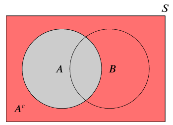
• Since \(A\) and \(A^c\) are disjoint, we have \(\mathbb{P}(A^c) = \mathbb{P}(S) - \mathbb{P}(A) = 1 - \mathbb{P}(A)\).

• Impossible events have probability zero: \(\mathbb{P}(\emptyset) = 0\).

• For (not necessarily disjoint) events \(A\) and \(B\), we have \(\mathbb{P}(A \cup B) = \mathbb{P}(A) + \mathbb{P}(B) - \mathbb{P}(A \cap B)\).

• If \(A \subseteq B\), then \(\mathbb{P}(A) \leq \mathbb{P}(B)\).

Suggested exercises: Q1 – Q10.

1.2 Counting principles

🔑 Key idea

When our experiment has \(m\) outcomes, each of which is equally likely, then each outcome \(s\) in the sample space \(S\) has probability \[\mathbb{P}(\{s\}) = \frac{1}{m} \] and each event \(A \subseteq S\) has probability \[ \mathbb{P}(A) = \frac{|A|}{m}=\frac{\text{number of ways A~can occur}}{\text{total no. of outcomes}}.\]

In this section, we look at some different ways to count the number of outcomes in an event, when the events are more complex than, say, a roll of a die.

1.2.1 The multiplication principle

If our experiment can be broken down into \(r\) smaller experiments, in which

• the first experiment has \(m_1\) equally likely outcomes

• the second experiment has \(m_2\) equally likely outcomes

• \(\cdots\)

• the \(r\)th experiment has \(m_r\) equally likely outcomes,

then there are \[\begin{aligned} m_1 \times m_2 \times \dots \times m_r = \prod_{j=1}^r m_j \end{aligned}\] possible, equally likely, outcomes for the whole experiment.

💪 Try it out

• If there are four different routes from Newcastle to Durham, and three different routes from Durham to York, how many different routes are there from Newcastle to York?

• If I toss six coins (1p, 2p, 5p, 10p, 15p, and 20p), how many different ways are there to get one ‘heads’ and five ‘tails’?

In general, sampling \(r\) times with replacement from \(m\) options gives \(m^r\) different possiblities.

1.2.2 Permutations

When we select \(r\) items from a group of size \(n\), in order and without replacement, we call the result a permutation of size \(r\) from \(n\).

🔑 Key idea

The number of permutations of size \(r\) from \(n\) is \[\begin{aligned} n \times (n-1) \times \dots \times (n-r+1) = \frac{n!}{(n-r)!}. \end{aligned}\]

A special case is when we want to arrange the whole list. Then, there are \[\begin{aligned} r \times (r-1) \times \dots \times 1 = \frac{r!}{0!} = r! \end{aligned}\] different permutations.

💪 Try it out

• How many different ways are there to arrange six books on a shelf?

• In a society with twenty members, which must choose one president and one secretary, how many different ways can these roles be filled?

• If six (six-sided) dice are rolled, what is the probability that each of the numbers 1-6 appears exactly once?

1.2.3 Combinations

When we select \(r\) items from a group of size \(n\), without replacement, but not in any particular order, then we have a combination of size \(r\) from \(n\).

🔑 Key idea

There are \[\begin{aligned} {n \choose r} = \frac{(n!)}{(n-r)! r!} \end{aligned}\] different ways to choose a combination of size \(r\) from \(n\) objects.

Two useful ways of thinking about combinations:

• You might notice that \({n \choose r} = {n \choose n-r}\). This is because we can also look at the combination of items we don’t pick. It’s much easier (psychologically, at least) to list the different ways to leave 3 cards in the deck than it is to list the different ways to draw 49 cards!

• There is a relationship between combinations and permutations: \[\begin{aligned} \text{the number of combinations} = \frac{1}{r!} \times \text{ the number of permutations}. \end{aligned}\] This is because each combination counted when the order doesn’t matter comes up \(r!\) different times when the order does matter.

💪 Try it out

• How many different ways are there to form a subcommittee of eight people, from a group of twenty?

• If I have \(n\) points on the circumference of a circle, how many different triangles can I form with vertices among these points?

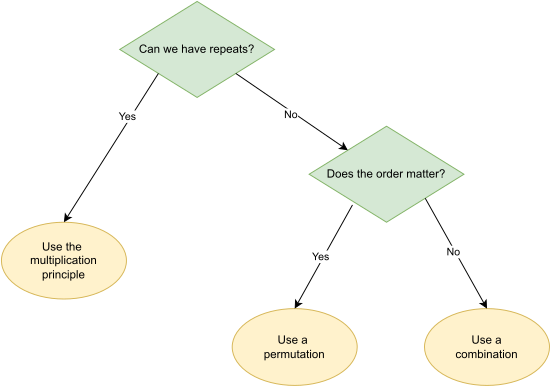
Remember: If we’re allowed repeated values, the only tool we need is the multiplication principle.

If there can be no repeats (sampling without replacement), then we use permutations if the objects are all distinct, and combinations if they are not. Usually if we’re dealt a hand of cards, or draw a bunch of things out of a bag, then they’re indistinguishable. But if we’re rolling several dice, or assigning objects to people, then we can (hopefully) tell the dice or people apart.

You might find the flowchart in Figure 1.3 helpful.

Figure 1.3: A decision-making flowchart for permutations, combinations, and the multiplication principle.

1.2.4 Multinomial coefficients

When we want to separate a group of size \(n\) into \(k \geq 2\) groups of possibly different sizes, we use multinomial coefficients.

🔑 Key idea

If the group sizes are \(n_1, n_2, \dots, n_k\), with \(n_1 + n_2 + \dots + n_k = n\), then the number of different ways to arrange the groups is given by the multinomial coefficient \[\begin{aligned} \binom{n}{n_1, n_2, \ldots, n_k} = \frac{n!}{n_1! n_2! \ldots n_k!}. \end{aligned}\]

To see how this works, think about choosing the groups in order. There are \(\binom{n}{n_1}\) ways to choose the first group; then, there are \(\binom{n-n_1}{n_2}\) ways to choose the second group from the remaining objects. Continuing like this until all the groups are selected, by the multiplication principle there are \[\begin{aligned} \binom{n}{n_1} \times \binom{n - n_1}{n_2} \times \binom{n - n_1 - n_2}{n_3} \times \dots \times \binom{n_{k-1} + n_k}{n_{k-1}} \times \binom{n_k}{n_k} \end{aligned}\] ways to choose all the groups. Writing each binomial coefficient in terms of factorials, and doing (lots of nice) cancelling, we end up with our expression for the multinomial coefficient.

As it turns out, the multinomial coefficient \(\binom{n}{n_1, n_2, \ldots, n_k}\) is also the number of different (i.e. distinguishable) permutations of \(n\) objects of which \(n_1\) are identical and of type 1, \(n_2\) are identical and of type 2, …, \(n_k\) are identical and of type \(k\) (where \(n = n_1 + n_2 + \dots + n_k\)).

Example

The number of different ways to distribute \(10\) toys among \(3\) children, ensuring that the youngest gets exactly one more than its older siblings, is \[\binom{10}{4, 3, 3} = \frac{10!}{4! 3! 3!} = 4,200.\]

💪 Try it out

• In how many different (i.e. distinguishable) ways can you arrange the letters in STATISTICS?

• If you arrange the letters S,S,S,T,T,T,I,I,A,C in a random order, what is the probability that they spell ‘Statistics’?

Suggested exercises: Q11 – Q17.

1.3 Conditional Probability and Bayes’ Theorem

Sometimes, knowing whether or not one event has occurred can change the probability of another event. For example, if we know that the score on a die was even, there is a one in three chance that we rolled a two (rather than one in six). Gaining the knowledge that our score is even affects how likely it is that we got each possible score.

Definition

We write \(\mathbb{P}(A \mid B)\) for the conditional probability of \(A\), given \(B\); it is defined by \[\begin{aligned} \mathbb{P}(A \mid B) = \frac{\mathbb{P} (A \cap B)}{\mathbb{P}(B)}. \end{aligned}\]

🔑 Key idea

We can rearrange the definition of conditional probability to get \[\begin{aligned} \mathbb{P}(A \cap B) = \mathbb{P}(A \mid B) \ \mathbb{P}(B) = \mathbb{P}(B \mid A) \ \mathbb{P}(A), \end{aligned}\] which leads to Bayes’ theorem: \[\begin{aligned} \mathbb{P}(A \mid B) = \frac{\mathbb{P} (B \mid A) \mathbb{P}(A)}{\mathbb{P}(B)}. \end{aligned}\]

Writing conditional probabilities in this way allows us to “invert” them; quite often, one of \(\mathbb{P}(A \mid B)\) and \(\mathbb{P}(B \mid A)\) is easier to spot than the other.

1.4 Independence

Definition

We say that two events are independent if the occurrence of one has no bearing on the occurrence of the other, that is, \[\begin{aligned} \mathbb{P}(A \mid B) = \mathbb{P}(A). \end{aligned}\]

Examples

• The scores obtained from rolling two separate dice are independent.

• Height and shoe size of people are usually not independent.

• Lecture attendance and exam grades are not independent!

When events \(A\) and \(B\) are independent, we have \[\begin{aligned} \mathbb{P}(A \cap B) = \mathbb{P}(A) \mathbb{P}(B). \end{aligned}\]

1.5 Partitions

Suppose we can separate our sample space into \(n\) mutually disjoint events \(E_1, E_2, \dots, E_n\): we know that exactly one of these events must happen. We call the collection \(\{ E_1, E_2, \dots, E_n\}\) a partition, and we can use it to break down the probabilities of different events \(A \subseteq S\).

First, we can write \[\begin{aligned} A = (A \cap E_1) \cup (A \cap E_2) \cup \dots \cup (A \cap E_n), \end{aligned}\] so that \[\begin{aligned} \mathbb{P}(A) = \mathbb{P}(A \cap E_1) + \mathbb{P}(A \cap E_2) + \dots + \mathbb{P}(A \cap E_n). \end{aligned}\] We can also introduce conditional probability, to get the partition theorem: \[\begin{aligned} \mathbb{P}(A) = \mathbb{P}(A \mid E_1)\ \mathbb{P}(E_1) + \mathbb{P}(A \mid E_2)\ \mathbb{P}(E_2) + \dots + \mathbb{P}(A \mid E_n)\ \mathbb{P}(E_n). \end{aligned}\] The partition theorem is useful whenever we can break an event down into cases, each of which is straightforward.

💪 Try it out

One of the most well-known (especially recently!) examples of the partition theorem is in testing for diseases.

Suppose that a disease affects one in 10,000 people. We have a test for this disease which correctly identifies 90% of people who do have the disease (so gives false negatives to 10% of people with the disease), and gives false positives to 1% of people who do not have the disease.

If a randomly chosen person is tested, what is the probability that their test result is positive?

Given that the test result is positive, what is the probability that they have the disease?

Suggested exercises: Q18 – Q26.

1.6 Random variables

Definition

A random variable \(X\) is a function \(X : S \to \mathbb{R}\) which assigns a numerical value to each possible outcome of an experiment (i.e. to each element of the sample space \(S\)), such that the probability \(\mathbb{P}(X \leq b)\) is well defined for all \(b \in \mathbb{R}\) (i.e. the event \(\{X \leq b\} = \mathbb{P}(\{s \in S \mid X(s) \leq b \}\) can always be assigned a probability).

We say that a random variable is discrete if we can list its possible values, or continuous if it can take any value in a range.

We won’t ever need to worry about the “well-defined” part of the definition in this module, but, strictly speaking, there do exist complicated real-valued functions on certain sample spaces which are not random variables.

Example

If the experiment is “toss four coins”, then some of the elements of the sample space are HHHH, HHHT, HHTH, HHTT,... . One random variable we can define is \[\begin{aligned} X = \text{ Number of heads}. \end{aligned}\] Then if our outcome is HHTT, we have \(X(\text{HHTT}) = 2\).

1.6.1 Discrete random variables

To describe a discrete random variable \(X : S \to \mathbb{R}\), we can use its probability distribution, which is sometimes called a probability mass function.

🔑 Key idea

The probability distribution is often displayed in a table, which shows the different values \(X\) can take, along with the associated probabilities:

values	\(x_1\)	\(x_2\)	…	\(x_n\)
probabilities	\(\mathbb{P}(X=x_1)\)	\(\mathbb{P}(X=x_2)\)	…	\(\mathbb{P}(X=x_n)\)

Recall here that the event \(\{X = x\}\) is given by \(\{X = x\} = \{s \in S \mid X(s) = x\} \subseteq S\). In a probability distribution, the probabilities must be non-negative and must sum to 1. To find the probability that \(X\) takes values in an interval \([a,b]\), we have \[\begin{aligned} \mathbb{P}(a \leq X \leq b) = \sum_{a \leq x_i \leq b} \mathbb{P}(X = x_i). \end{aligned}\]

1.6.1.1 Joint and marginal distributions

Definition

When we have two (or more) discrete random variables, \(X\) and \(Y\) (and \(Z\) and...), the joint probability distribution is the table of probabilities \(\mathbb{P}(X=x, Y=y)\) of every possible combination of values \(x\) for \(X\) and \(y\) for \(Y\):

	\({x_1}\)	…	\({x_n}\)
\({y_1}\)	\(\mathbb{P}(X=x_1, Y=y_1)\)	…	\(\mathbb{P}(X=x_n,Y=y_1)\)
\(\vdots\)	\(\vdots\)	\(\ddots\)	\(\vdots\)
\({y_m}\)	\(\mathbb{P}(X=x_1,Y=y_m)\)	…	\(\mathbb{P}(X=x_n,Y=y_m)\)

Recall here that the event \(\{X = x, Y=y\}\) is given by \(\{X = x, Y=y\} = \{X=x\} \cap \{ Y= y\} \subseteq S\). Moreover, as in the case of the probability distribution of a single random variable, the probabilities in a joint probability distribution must be non-negative and must sum to 1.

We can find the marginal probability distributions of \(X\) and \(Y\) from the joint distribution, by summing across the rows or columns: \[\begin{aligned} \mathbb{P}(X=x_k) =\sum_{j} \mathbb{P}(X=x_k,Y=y_j), \\ \mathbb{P}(Y=y_j) =\sum_{k} \mathbb{P}(X=x_k,Y=y_j). \end{aligned}\]

Two discrete random variables \(X\) and \(Y\) are said to be independent if \[\mathbb{P}(X = x_k, Y = y_j) = \mathbb{P}(X = x_k) \, \mathbb{P}(Y = y_j)\] for all possible pairs \((x_k, y_j)\) of values of \(X\) and \(Y\).

💪 Try it out

Let \(X\) be the random variable which takes value \(3\) when a fair coin lands heads up, and takes value \(0\) otherwise. Let \(Y\) be the value shown after rolling a fair die. Write down the distributions of \(X\) and \(Y\), and the joint distribution of \(X\) and \(Y\). You may assume that \(X\) and \(Y\) are independent. Use your table to find the probability that \(X>Y\).

Example

Let \(S = \{(a,b) \mid a,b \in \{1, \dots, 6\}\}\) be the sample space when a pair of fair dice is tossed. Let \(X : S \to \mathbb{R}\) and \(Y : S \to \mathbb{R}\) be the (discrete) random variables defined by \[X(a,b) = a+b \quad \text{and} \quad Y(a,b) = \max\{a,b\}\] respectively. Then the joint distribution of \(X\) and \(Y\) is

	\(2\)	\(3\)	\(4\)	\(5\)	\(6\)	\(7\)	\(8\)	\(9\)	\(10\)	\(11\)	\(12\)
\(1\)	\(\tfrac{1}{36}\)	\(0\)	\(0\)	\(0\)	\(0\)	\(0\)	\(0\)	\(0\)	\(0\)	\(0\)	\(0\)
\(2\)	\(0\)	\(\tfrac{2}{36}\)	\(\tfrac{1}{36}\)	\(0\)	\(0\)	\(0\)	\(0\)	\(0\)	\(0\)	\(0\)	\(0\)
\(3\)	\(0\)	\(0\)	\(\tfrac{2}{36}\)	\(\tfrac{2}{36}\)	\(\tfrac{1}{36}\)	\(0\)	\(0\)	\(0\)	\(0\)	\(0\)	\(0\)
\(4\)	\(0\)	\(0\)	\(0\)	\(\tfrac{2}{36}\)	\(\tfrac{2}{36}\)	\(\tfrac{2}{36}\)	\(\tfrac{1}{36}\)	\(0\)	\(0\)	\(0\)	\(0\)
\(5\)	\(0\)	\(0\)	\(0\)	\(0\)	\(\tfrac{2}{36}\)	\(\tfrac{2}{36}\)	\(\tfrac{2}{36}\)	\(\tfrac{2}{36}\)	\(\tfrac{1}{36}\)	\(0\)	\(0\)
\(6\)	\(0\)	\(0\)	\(0\)	\(0\)	\(0\)	\(\tfrac{2}{36}\)	\(\tfrac{2}{36}\)	\(\tfrac{2}{36}\)	\(\tfrac{2}{36}\)	\(\tfrac{2}{36}\)	\(\tfrac{1}{36}\)

For example, the event that both \(X=5\) and \(Y=3\) occurs only for the outcomes \((2,3)\) and \((3,2)\), yielding a probability \(\mathbb{P}(X=5, Y=3) = \frac{2}{36}\). The (marginal) probability that \(X=5\) is \[\begin{aligned} \mathbb{P}(X=5) &= \sum_{k=1}^6 \mathbb{P}(X=5, Y=k) \\ &= \mathbb{P}(X=5, Y=3) + \mathbb{P}(X=5, Y=4) \\ &= \frac{2}{36} + \frac{2}{36} = \frac{4}{36} \end{aligned}\] as expected, since \(X=5\) occurs only for the outcomes \((1,4), (2,3), (3,2)\) and \((4,1)\). Similarly, the (marginal) probability that \(Y=3\) is \[\begin{aligned} \mathbb{P}(Y=3) &= \sum_{m=2}^{12} \mathbb{P}(X=m, Y=3) \\ &= \mathbb{P}(X=4, Y=3) + \mathbb{P}(X=5, Y=3) + \mathbb{P}(X=6, Y=3) \\ &= \frac{2}{36} +\frac{2}{36} +\frac{1}{36} = \frac{5}{36} \end{aligned}\] since \(Y=3\) occurs only for the outcomes \((1,3), (2,3), (3,3), (3,2)\) and \((3,1)\).

Finally, observe that \(X\) and \(Y\) are not independent random variables since, for example, \(\mathbb{P}(X=2, Y=3) = 0\), whereas \(\mathbb{P}(X=2) = \frac{1}{36}\) and \(\mathbb{P}(Y=3) = \frac{5}{36}\), so that \(\mathbb{P}(X=2)\, \mathbb{P}(Y=3) \neq 0\).

1.6.2 Continuous random variables

When our random variable is continuous, we cannot describe its probability distribution using a list of probabilities. Instead, we use a probability density function (pdf), \(f_X(x)\).

🔑 Key idea

The density function \(f_X(x)\) describes a curve over the possible values taken by the random variable \(X\). In a density function, the values must be non-negative and integrate to 1.

To find the probability that \(X\) lies in an interval \([a,b]\), we have \[\begin{aligned} \mathbb{P}(a \leq X \leq b) = \int_a^b f_X(x) \, dx. \end{aligned}\]

Remember that the density \(f_X(x)\) is not the same thing as \(\mathbb{P}(X=x)\). In fact, for every \(x\), we have \(\mathbb{P}(X=x) = 0\).

Another way of specifying the distribution of a continuous random variable is through its cumulative distribution function (cdf) \(F_X : \mathbb{R} \to [0,1]\), given by \[\begin{aligned} F_X(x) = \mathbb{P}(X \leq x) = \int_{-\infty}^x f_X(t) \, dt. \end{aligned}\]

Example

A random variable \(X\) is said to have a uniform distribution (often denoted Unif\((a,b)\)) on an interval \([a,b]\) if its probability density function \(f_X\) satisfies \[f_X(x) = \begin{cases} \frac{1}{b-a} \,, & \text{for } x \in [a,b]\,, \\ 0\,, & \text{otherwise.} \end{cases}\] If \([c,d] \subset [a,b]\) is another interval (that is, if \(a \leq c < d \leq b\)), then \[\mathbb{P}(c \leq X \leq d) = \int_c^d f_X(x) \, dx = \frac{1}{b-a}\int_c^d dx = \frac{d-c}{b-a}\,.\] Similarly, if the interval \([c', d']\) has \(c' < a \leq d' \leq b\), then, since \(f_X(x) = 0\) for all \(x < a\), \[\mathbb{P}(c' \leq X \leq d') = \int_{c'}^{d'} f_X(x) \, dx = \int_{a}^{d'} f_X(x) \, dx = \frac{1}{b-a}\int_a^{d'} dx = \frac{d'-a}{b-a}\,.\] Via similar calculations, we see that the cumulative distribution function \(F_X : \mathbb{R} \to [0,1]\) is given by \[F_X(x) = \begin{cases} 0, & \text{for } x < a, \\ \frac{x - a}{b-a} \,, & \text{for } a \leq x \leq b, \\ 1\,, & \text{for } b < x. \end{cases}\]

💪 Try it out

Let \(X\) be a continuous random variable with probability density function: \[f_X(x) = \begin{cases} \beta e^{-\beta x}\,, & \text{for}~x>0,\\ 0\,, & \text{for}~x\leq 0. \end{cases}\] Check that \(f_X(x)\) is a valid probability density function when \(\beta>0\). Find the cumulative distribution function of \(X\) and, hence, find \(\mathbb{P}(X>3)\).

1.6.2.1 Joint and marginal distributions

Definition

The joint probability distribution of two (or more) continuous random variables \(X\) and \(Y\) (and \(Z\) and...) can be described using their joint probability density function \(f_{X,Y}(x,y)\). This is a function of two variables describing how the pair of random variables \(X\) and \(Y\) are “spread out”.

As it is a density, the function \(f_{X,Y}\) is non-negative and must integrate to 1. The probability that \(X\) and \(Y\) take values in a region \(A\) of the \(xy\)-plane is given by the double integral (to be discussed in ?sec-integration \[\label{E:jpdf} \mathbb{P}( (X,Y) \in A) = \iint_A f_{X,Y}(x,y) \, dx dy.\]

We can find the marginal probability distributions of \(X\) and \(Y\) from the joint distribution, by integrating out one of the variables: \[\begin{aligned} f_X(x) = \int_{-\infty}^\infty f_{X,Y}(x,y) \, dy \\ f_Y(y) = \int_{-\infty}^\infty f_{X,Y}(x,y) \, dx. \end{aligned}\]

Suggested exercises: Q27 – Q32.

1.7 Expectation and Variance

While the probability distribution or probability density function tells us everything about the distribution of a random variable, this can often be too much information. Quantities which instead summarise the distribution can be useful to convey information about our random variable without trying to describe it in its entirity.

Summaries of a distribution include the expectation, the variance, the skewness and the kurtosis. In this course, we’re only interested in the expectation, which tells us about the location of the distribution, and the variance, which tells us about its spread. The skewness tells us about the symmetry of the distribution about its expectation, while the kurtosis tells us about the likelihood of the random variable taking values far away from the mean.

1.7.1 Expectation

Definition

The expectation of a random variable \(X\) is given by \[\mathbb{E}[X] = \begin{cases} \sum_x x \, \mathbb{P}(X=x) \,, & \text{if $X$ is discrete,} \\[3mm] \int_{-\infty}^\infty x f_X(x) \, dx \,, & \text{if $X$ is continuous.} \end{cases}\] The expectation is sometimes called the mean or the average of the random variable \(X\).

1.7.1.1 Properties of Expectation

Linearity: If \(X\) is a random variable and \(a\) and \(b\) are (real) constants, then \[\begin{aligned} \mathbb{E}[aX + b] = a \, \mathbb{E}[X] + b. \end{aligned}\]

Additivity: If \(X_1, X_2, \dots, X_n\) are random variables, then \[\begin{aligned} \mathbb{E}[X_1 + X_2 + \dots + X_n] = \mathbb{E}[X_1] + \mathbb{E}[X_2] + \dots + \mathbb{E}[X_n]. \end{aligned}\]

Positivity: If \(X\) is a positive random variable (that is, if \(\mathbb{P}(X \geq 0) = 1\)), then \(\mathbb{E}[X] \geq 0\).

Independence: If \(X\) and \(Y\) are independent random variables, then \[\begin{aligned} \mathbb{E}[XY] = \mathbb{E}[X] \, \mathbb{E}[Y]. \end{aligned}\]

Expectation of a function: If \(X\) is a random variable and \(r\) is a (nice¹) function, then \(r(X) = r \circ X\) is a random variable with expectation \[\mathbb{E}[r(X)] = \begin{cases} \sum_{x} r(x)\, \mathbb{P}(X=x) \,, & \text{if $X$ is discrete,} \\[3mm] \int_{-\infty}^\infty r(x) f_X(x) \, dx \,, & \text{if $X$ is continuous.} \end{cases}\]

1.7.2 Variance

Definition

For a random variable \(X\) with expectation \(\mathbb{E}[X] = \mu\), the variance of \(X\) is given by \[\begin{aligned} \text{Var}(X) = \mathbb{E}[(X - \mu)^2]. \end{aligned}\]

By expanding out the brackets and using the linearity of the expectation, we can rewrite the variance as \[\begin{aligned} \text{Var}(X) = \mathbb{E}[X^2] - \mathbb{E}[X]^2. \end{aligned}\]

The variance is always positive, because it is the expectation of a positive random variable. The standard deviation is the square root of the variance: \[\begin{aligned} \sigma_X = \sqrt{\text{Var}(X)}. \end{aligned}\]

1.7.2.1 Properties of Variance

Affine transformations: If \(X\) is a random variable and \(a\) and \(b\) are (real) constants, then \[\begin{aligned} \text{Var}(aX + b) = a^2 \text{Var}(X). \end{aligned}\]

Independence: If \(X\) and \(Y\) are independent random variables, then \[\begin{aligned} \text{Var}(X + Y) = \text{Var}(X) + \text{Var}(Y). \end{aligned}\]

💪 Try it out

• Let \(X\) be a continuous random variable with probability density function: \[\begin{aligned} f_X(x) &= \left\{ \begin{array}{ll} \beta e^{-\beta x} & \text{for}~x>0,\\ 0 & \text{for}~x\leq 0.\end{array}\right. \end{aligned}\] What are the expectation and variance of \(X\)?

• Let \(Y\) be a random variable with the following probability distribution:

\(y\)	\(1\)	\(2\)	\(3\)
\(\mathbb{P}(Y=y)\)	\(\frac16\)	\(\frac26\)	\(\frac36\)

Find \(\mathbb{E}[X]\), \(\text{Var}(X)\), and \(\mathbb{E}\left[\frac1X\right]\).

Suggested exercises: Revisit Q30; Q33 – Q37.

1.8 The Binomial Distribution

Definition

If \(X\) is the number of successes (i.e. 0 or 1) from a single experiment which succeeds with probability \(p\) and fails with probability \(1-p\), then the random variable \(X\) has probability distribution

              $x$   $0$    $1$
------------------ ------- -----
$\mathbb{P}(X=x)$  $1-p$   $p$

In such a case, we say that \(X\) has a Bernoulli distribution with parameter \(p\) and write \(X \sim \text{Bern}(p)\).

The expectation and variance of \(X \sim \text{Bern}(p)\) are: \[\begin{aligned} \mathbb{E}[X] & = p \\ \text{Var}(X) & = p(1-p). \end{aligned}\]

Suppose we have \(n\) Bernoulli-style trials, which succeed or fail independently of each other, and such that all trials have the same probability \(p\) of succeeding. We count the total number of successes across all the trials.

Definition

If \(Y\) is the total number of successes from \(n\) independent Bernoulli trials (each with parameter \(p\)), we say that \(Y\) has a binomial distribution with parameters \(n\) and \(p\), and we write \(Y \sim \text{Bin}(n,p)\).

If \(0 \leq k \leq n\), we have \[\begin{aligned} \mathbb{P}(Y = k) = \binom{n}{k} p^k (1-p)^{n-k}. \end{aligned}\] This is because each configuration of \(k\) successes and \(n-k\) successes has probability \(p^k (1-p)^{n-k}\), by the multiplication principle; and there are \(\binom{n}{k}\) different ways of arranging the \(k\) successes and \(n-k\) failures among the trials.

💪 Try it out

Check that the probabilities in the binomial distribution are all non-negative and sum to 1.

The expectation and variance of \(Y \sim \text{Bin}(n,p)\) are: \[\begin{aligned} \mathbb{E}[Y] &= np \\ \text{Var}(Y) &= np(1-p). \end{aligned}\]

Examples

• If I toss six coins, the total number of heads has a \(\text{Bin}(6, \frac{1}{2})\) distribution.

• If each SMB student decides to skip a lecture with probability 0.2, then the number of students who turn up has a \(\text{Bin}(217, 0.8)\) distribution (assuming you all decide independently of each other!). In particular, the expected number of students at each lecture is \(217 \times 0.8 \approx 174\).

1.9 The Poisson Distribution

While the binomial distribution is about counting successes in a fixed number of trials, the Poisson distribution lets us count how many times something happens without a fixed upper limit. This is useful in a lot of real-world contexts, for example:

• the number of people who visit a website

• the number of yeast cells in a sample (such as in experiments by Gossett at Guinness in the 1920s)

• the number of particles emitted from a radioactive sample.

Definition

The Poisson distribution is used to model scenarios in which events happen randomly, independently, and at a constant rate \(r\). If \(X\) is the total number of these events that happen in a time period of length \(s\), then \(X\) has a Poisson distribution with parameter \(\lambda = rs\), and we write \(X \sim \text{Po}(\lambda)\).

If \(k \in \mathbb{N}\), we have \[\begin{aligned} \mathbb{P}(X=k) = e^{-\lambda} \frac{\lambda^k }{k!}. \end{aligned}\]

💪 Try it out

Check that the probabilities in the Poisson distribution are all non-negative and sum to 1.

The expectation and variance of \(X\) are \[\begin{aligned} \mathbb{E}[X] = \text{Var}(X) = \lambda. \end{aligned}\]

1.9.1 Using the Poisson distribution to approximate the binomial distribution

Instead of thinking about our time period \([0,s]\) as one long interval, we can split it up into \(n\) smaller ones (each one will have length \(\frac{s}{n}\)).

Suppose we count the number of sub-intervals in which events occur. If the sub-intervals are small enough, it is very unlikely that there will be multiple events in any of them, and the probability that there is one event will be \(p \approx \frac{rs}{n} = \frac{\lambda}{n}\).

We can view the sub-intervals as \(n\) independent trials, and the total number of successes becomes binomially distributed.

This is a good approximation because the probabilities \(\mathbb{P}(X=k)\) in the binomial distribution \(\text{Bin}(n, \frac{\lambda}{n})\) and the Poisson distribution \(\text{Po}(\lambda)\) are similar as long as \(n\) is big enough. That is, for large \(n\) we have \[\begin{aligned} \binom{n}{k} \left( \frac{\lambda}{n}\right)^k \left( 1 - \frac{\lambda}{n} \right)^{n-k} & = \frac{ n(n-1) \dots (n-k+1)}{k!} \frac{\lambda^k}{n^k} \left( 1 - \frac{\lambda}{n} \right)^{n-k} \\ & = \frac{ n(n-1) \dots (n-k+1)}{n^k} \times \left( 1 - \frac{\lambda}{n} \right)^{n-k} \times \frac{\lambda^k}{k!} \\ & \approx 1 \times e^{-\lambda} \times \frac{\lambda^k}{k!}, \end{aligned}\]

This approximation is good if \(n \geq 20\) and \(p \leq 0.05\), and excellent if \(n \geq 100\) and \(np \leq 10\).

Suggested exercises: Revisit Q38–Q41.

1.10 The Normal Distribution

Unlike the binomial and Poisson distributions, the normal (or Gaussian) distribution is continuous. It is one of the most used (and most useful) distributions. A random variable whose “large-scale” randomness comes from many small-scale contributions is usually normally distributed: for example, people’s heights are determined by many different genetic and environmental factors. All of these different factors have tiny impacts on your final height; overall, the distribution of the height of a random person is roughly normal.

1.10.1 The standard normal distribution

The first version of the normal distribution we will meet is the standard normal.

Definition

We say that a continuous random variable \(Z\) has a standard normal distribution, and we write \(Z \sim \mathcal{N}(0,1)\), if its probability density function is given by \[f_Z(x) = \frac{1}{\sqrt{2\pi}} e^{-\frac{x^2}{2}}\] for all \(x \in \mathbb{R}\).

Properties of the standard normal distribution

• The probability density function \(f_Z\) of a random variable with standard normal distribution is symmetric about 0. Then \[\mathbb{P}(Z \leq z) = \mathbb{P}(Z \geq - z) = \mathbb{P}(-Z \leq z),\] which implies, in particular, that the random variable \(-Z\) has the same (normal) distribution as \(Z\).

• This symmetry also means that \(x f_Z(x)\) is an odd function; so the expectation of \(Z\) is zero.

• The variance of \(Z\) is \[\begin{aligned} \text{Var}(Z) & = \mathbb{E}[Z^2] - 0 \\ & = \int_{-\infty}^{\infty} x^2 f_Z(x) \, dx \\ & = \frac{1}{\sqrt{2\pi}} \int_{\infty}^{\infty} x^2 e^{-\frac{x^2}{2}} \, dx = 1. \end{aligned}\] (You can find this via integration by parts.)

The cumulative distribution function for \(Z\)

Definition

The cumulative distribution function for \(Z\) is denoted \(\Phi(z)\) and is given by \[\begin{aligned} \Phi(z) = \mathbb{P}(Z \leq z) = \int_{-\infty}^z \frac{1}{\sqrt{2\pi}} e^{-\frac{x^2}{2}} \, dx. \end{aligned}\]

There is no neat (“algebraic”) expression for \(\Phi(z)\): in practice, when we need to evaluate it we use numerical methods to get (usually very good) approximations. These values are traditionally recorded in tables but usually, they’re built into computer software and some calculators.

Some useful properties of \(\Phi(z)\), which reduce the number of values we need in the tables, are:

• Because \(f_Z(x)\) is symmetric, we have \[\Phi(z) = \mathbb{P}(Z \leq z) = \mathbb{P}(Z \geq - z) = 1 - \Phi(-z) \,.\]

• We have \(\Phi(0) = \frac{1}{2}\).

• \(\mathbb{P}(a \leq Z \leq b) = \Phi(b) - \Phi(a)\).

Interpolation: When the value we need to find isn’t in a table we have access to, we can interpolate. If \(a < b < c\) and we know \(\Phi(a)\) and \(\Phi(b)\), we approximate: \[\begin{aligned} \Phi(b) \approx \Phi(a) + \frac{b-a}{c-a} \left(\Phi(c) - \Phi(a) \right). \end{aligned}\]

For example, most normal tables only go to two decimal places, but \(\Phi(0.553)\) will be approximately \((0.553 - 0.55)/(0.56-0.55) = 0.3\) of the way between \(\Phi(0.55)\) and \(\Phi(0.56)\).

1.10.2 General normal distributions

Definition

We say that a continuous random variable \(X\) has a normal distribution with parameters \(\mu\) and \(\sigma^2\), and we write \(X \sim \mathcal{N}(\mu, \sigma^2)\), if the random variable \(Z = \frac{X-\mu}{\sigma}\) has a standard normal distribution.

We can also write this in the other direction: \(X \sim \mathcal{N}(\mu, \sigma^2)\) if \(X = \sigma Z + \mu\). Since the distribution of \(Z\) is symmetric, we use the convention \(\sigma > 0\).

Properties of general normal distributions

• The expectation of \(X\) is \[\begin{aligned} \mathbb{E}[X] &= \mathbb{E}[\sigma Z + \mu] \\ &= \mu + \sigma \, \mathbb{E}[Z] \\& = \mu + 0 = \mu. \end{aligned}\]

• The variance of \(X\) is \[\begin{aligned} \text{Var}(X) & = \text{Var}(\sigma Z + \mu) \\ & = \sigma^2 \, \text{Var}(Z) \\ & = \sigma^2. \end{aligned}\]

• The probability density function of \(X\) is \[\begin{aligned} f_X(x) = \frac{1}{\sigma} f_Z\left(\frac{x-\mu}{\sigma} \right) = \frac{1}{\sigma \sqrt{ 2 \pi}} \exp \left\{ -\frac{1}{2} \left( \frac{x-\mu}{\sigma} \right)^2 \right\}. \end{aligned}\]

• The cumulative distribution function of \(X\) is given by \[\begin{aligned} \mathbb{P}(X \leq x) & = \mathbb{P} \left( \sigma Z + \mu \leq \frac{x-\mu}{\sigma} \right) \\ & = \mathbb{P}\left(Z \leq \frac{x-\mu}{\sigma}\right) \\ & = \Phi\left( \frac{x-\mu}{\sigma} \right). \end{aligned}\] We can use the table for the standard normal distribution to evaluate the cumulative distribution function of any normal distribution, by using this transformation.

💪 Try it out

1. If \(X \sim \mathcal{N}(12,25)\), what is \(\mathbb{P}(X \leq 3)\)?

2. If \(Y \sim \mathcal{N}(1,4)\), what is \(\mathbb{P}(-1 < Y < 2)\)?

1.10.3 Using the normal distribution to approximate the binomial and Poisson distributions

Just as we can use the Poisson distribution to approximate specific probabilities in the binomial distribution, we can use the normal distribution to approximate cumulative probabilities. If \(n\) is large and \(X \sim \text{Bin}(n,p)\), then approximately we have \(X \sim \mathcal{N}(np, np(1-p))\).

In particular, \[\mathbb{P}(X \leq k) \approx \Phi\left( \frac{ k-np}{\sqrt{np(1-p)}} \right).\]

This is a useful approximation when both \(np\) and \(np(1-p)\) are at least 10; as the two values increase, the approximation gets better.

💪 Try it out

A machine produces \(n = 1500\) gadgets every day. Each individual gadget is defective with probability \(p= 0.02\). Find (approximately) the probability that more than 40 of the items produced in one day are defective.

Similarly, we can use the normal distribution to approximate the cumulative probabilities in the Poisson distribution: if \(X \sim \text{Po}(\lambda)\), then approximately we have \(X \sim \mathcal{N}(\lambda, \lambda)\) and \[\mathbb{P}(X \leq k) \approx \Phi \left( \frac{k-\lambda}{\sqrt{\lambda}} \right).\]

This is a useful approximation when \(\lambda\) is at least 5, and gets better as \(\lambda\) increases.

Suggested exercises: Q42 – Q45.

1.11 The Central Limit Theorem

1.11.1 Experimental errors

Definition

When we are measuring a quantity whose “true value” is \(\mu\), our measurement takes the form \(X = \mu + \varepsilon\), where \(\varepsilon\) is the experimental error. Before we do the experiment, we can think of both \(\varepsilon\) and \(X\) as random quantities. Afterwards, \(X\) is a fixed and known quantity, and \(\mu\) and \(\varepsilon\) are fixed but unknown quantities (to us). Our goal is to use \(X\) to infer something about \(\mu\).

Assumption: We will assume that there are no systematic errors or bias in the experiment; in other words, \(\mathbb{E}[\varepsilon] = 0\).

If the variance of \(\varepsilon\) is \(\text{Var}(\varepsilon) = \sigma^2\), then \[\begin{aligned} \mathbb{E}[X] &= \mu + \mathbb{E}[\varepsilon] = \mu + 0 = \mu \\ \text{Var}(X) &= 0 + \text{Var}(\varepsilon) = \sigma^2. \end{aligned}\] This means that, on average, the value of our measurement is a good estimate of the value of \(\mu\); however,if the variance of \(\varepsilon\) is large, our measurement will have quite a high probability of being far from the true value.

To improve our estimate, we can do one of two things:

• try to improve our measurement technique, to reduce the variance

• take more measurements!

1.11.2 The sample mean

Definition

When we take \(n\) independent random variables \(X_1, X_2, \dots, X_n\) which all have the same distribution, we say that \(X_1, X_2, \dots, X_n\) are independent and identically distributed (i.i.d.).

Example

We might obtain i.i.d. samples by repeating our measurement, or experiment, \(n\) times, or by sampling \(n\) people from a large population.

Definition

If \(X_1, X_2, \dots, X_n\) are random variables, then the sample mean is the average \[\overline{X} = \frac1n \sum_{j=1}^n X_j.\]

Before we take our measurements, this is also a random variable; afterwards, it is just a number. To distinguish between the two situations, we use \(\overline{X}\) for the random variable, and \(\overline{x}\) for the number.

It is perhaps worth remarking that the definition of the sample mean is a little ambiguous, as \(\overline X\) is not defined on the same sample space as \(X_1, X_2, \dots, X_n\). Indeed, if \(S\) is the sample space on which each \(X_j\) is defined (i.e. \(X_j : S \to \mathbb{R}\)), then the sample mean is defined on the \(n\)-fold product sample space \(S \times S \times \dots \times S\) via \(\overline X(s_1, s_2, \dots, s_n) = \frac{1}{n} \sum_{j=1}^n X_j(s_j)\). That is, we take the list \((s_1, s_2, \dots, s_n) \in S \times S \times \dots \times S\) of \(n\) outcomes (e.g. of an experiment repeated \(n\) times), then evaluate the \(j^\text{th}\) random variable \(X_j\) on the \(j^\text{th}\) outcome \(s_j\) and, finally, compute the average of the values obtained. Let’s look at an example.

💪 Try it out

We toss a pair of fair dice eight times. For each toss, the sample space is given by \(S = \{(a,b) \mid a,b \in \{1, \dots, 6\}\}\). Let \(X_1, X_2, \dots, X_8\) be random variables, where \(X_j : S \to \mathbb{R}\) is defined as the sum \(X_j(a_j, b_j) = a_j + b_j\) of the outcome \((a_j, b_j) \in S\) of the \(j^\text{th}\) toss. If the outcomes of the eight tosses are \[(1,3), (5,2), (3,3), (5,6), (1,1), (4,3), (2,3) \text{ and }(1,3)\], respectively, find the sample and population means.

Answer: The sample mean (i.e. its value after all tosses have been completed) is given by \[\begin{aligned} \overline x &= \frac{1}{8}\left(X_1(1,3) + X_2(5,2) + X_3 (3,3) + X_4 (5,6) + X_5 (1,1) + X_6 (4,3) + X_7 (2,3) + X_8(1,3) \right) \\ &= \frac{1}{8} \, (4 + 7 + 6 + 11 + 2 + 7 + 5 + 4) \\ &= \frac{46}{8} = 5.75. \end{aligned}\]

On the other hand, the population mean/expectation in this case would be \(\frac{252}{36} = 7\), since the total of the sums \(a + b\) of all \(36\) possible outcomes \((a,b) \in S\) is \(252\). (It’s not hard to check directly that \(\mathbb{E}[X_j] = 7\) for each \(j\).) With a much larger number of tosses, we could expect that the sample mean would be close to the population mean/expectation.

Assumption: We assume that \(X_1, X_2, \dots, X_n\) are i.i.d. with shared mean \(\mu\) and variance \(\sigma^2\). Then \[\begin{aligned} \mathbb{E}[\overline{X}] & = \frac1n \sum_{j=1}^n \mathbb{E}[X_j] = \frac{n}{n} \mu = \mu \\ \text{Var}(\overline{X}) & = \frac1{n^2} \sum_{j=1}^n \text{Var}(X_j) = \frac{n}{n^2} \sigma^2 = \frac{\sigma^2}{n}. \end{aligned}\]

So the expectation of the sample mean is always \(\mu\): we call it an unbiased estimator for the mean. On the other hand, the variance is always smaller than \(\sigma^2\) , and decreases as we increase \(n\). By taking a large enough sample size, we can get as small a variance as we want.

If \(n\) is large enough, the sample mean will give an accurate estimate for the true mean \(\mu\). This result is called the Law of Large Numbers, which says that \(\overline{X}\) converges² to \(\mu\) as \(n \to \infty\).

1.11.3 The Central Limit Theorem

We know that the sample mean will be quite close to the true value \(\mu\) on average. The Central Limit Theorem tells us more about the distribution of the error.

🔑 Key idea: The Central Limit Theorem

If \(X_1, X_2, \dots, X_n\) are i.i.d. random variables with shared mean \(\mu\) and variance \(\sigma^2\), then, for large \(n\), the sample mean \(\overline{X}\) is approximately normally distributed with mean \(\mu\) and variance \(\frac{\sigma^2}{n}\); that is, \(\overline{X}\) is approximated by \(\mathcal{N}(\mu, \frac{\sigma^2}{n})\).

In other words, for large \(n\), the random variable \[Z = \frac{\overline{X} - \mu}{\frac{\sigma}{\sqrt{n}}}\] is approximately a standard normal distribution.

Here, when we say that the distribution is approximately normal, we mean that \[\mathbb{P}(a \leq \overline{X} \leq b ) \approx \Phi \left( \frac{b-\mu}{\sigma/\sqrt{n}} \right) - \Phi \left( \frac{a-\mu}{\sigma/\sqrt{n}} \right),\] whatever the values of \(a\) and \(b\).

💪 Try it out

• If the random variables \(X_1, X_2, \dots, X_{10}\) are independent, and all are uniformly distributed on the interval \([0, 1]\), use the Central Limit Theorem to estimate \(\mathbb{P}(X_1 + X_2 + \dots + X_{10} > 7)\).

• A manufacturing process is designed to produce bolts with a 0.5cm diameter. Once a day, a random sample of 36 bolts is selected and the diameters recorded. If the average of the 36 values is less than 0.49cm or greater than 0.51cm, then the process is shut down for inspection and adjustment. The standard deviation for individual diameters is 0.02cm. Find approximately the probability that the line will be shut down unnecessarily (i.e., if the true process mean really is 0.5cm).

Suggested exercises: Q46–Q50.

---

1. Here ‘nice’ actually means ‘measurable’. It’s possible to come up with functions \(r\) for which this doesn’t work; luckily for us, they’re usually quite weird and we won’t run into any of them.

2. There’s quite a lot of probability theory hiding behind this “converges”!