$$ \usepackage{derivative} \newcommand{\odif}[1]{\mathrm{d}#1} \newcommand{\odv}[2]{\frac{ \mathrm{d}#1}{\mathrm{d}#2}} \newcommand{\pdv}[2]{\frac{ \partial#1}{\partial#2}} \newcommand{\th}{\theta} \newcommand{\p}{\partial} \newcommand{\var}[1]{\text{Var}\left(#1\right)} \newcommand{\sd}[1]{\sigma\left(#1\right)} \newcommand{\cov}[1]{\text{Cov}\left(#1\right)} \newcommand{\cexpec}[2]{\mathbb{E}\left[#1 \vert#2 \right]} $$
3 Applications of Partial Derivatives
In this chapter we will discuss a few applications of partial derivatives.
3.1 The chain rule in multiple variables
Suppose we have functions \(f(x)\) and \(g(x)\), each depending on a single variable. Then we can compose them to get either a function \((f \circ g)(x) = f(g(x))\) (first do \(g\), then do \(f\)) or a function \((g \circ f)(x) = g(f(x))\) (first do \(f\), then do \(g\)), each of which also depends on only one variable. For example, the functions \(f(x) = x^2\) and \(g(x) = \sin (x)\) can be composed in to give either \((f \circ g)(x) = f(g(x)) = (\sin(x))^2\) (first \(g\), then \(f\)) or \((g \circ f)(x) = g(f(x)) = \sin(x^2)\) (first \(f\), then \(g\)).
Recall that the chain rule (in one variable) tells us how to differentiate compositions of functions (of one variable). More precisely, recall that \[\odv{}{x} (f \circ g)(x) = \odv{}{x} f((g(x)) = f'(g(x)) \, g'(x).\] You might be more familiar with thinking about the chain rule in the following (equivalent) way, which is perhaps more aesthetically pleasing (because we can imagine “canceling the ‘\(\odif{x}\)’”): suppose you have a function \(f(x)\) and suppose that the variable \(x\) also depends on another variable \(t\) (so that we have function \(x(t)\)). Then we can write the chain rule as \[\odv{f}{t} = \odv{f}{x} \odv{x}{t}\,.\] We can derive this formula by noting that the total differentials of \(f(x)\) and \(x(t)\) are given by \[\odif{f} = \odv{f}{x} \odif{x} \qquad \text{ and } \qquad \odif{x} = \odv{x}{t} \odif{t},\] which can then be combined to yield \[\odif{f} = \odv{f}{x} \odv{x}{t} \odif{t}.\] Dividing across by \(\odif{t}\) now gives us the chain rule \[\odv{f}{t} = \odv{f}{x} \odv{x}{t}\,.\]
If we want to generalise the chain rule to functions \(f(x_1, x_2, \dots, x_n)\) of several variables, there are two scenarios we need to deal with:
all the variables \(x_1, x_2, \dots, x_n\) are functions of a single variable \(t\); i.e. we have a composition \(f(x_1(t), x_2(t), \dots, x_n(t))\) depending on a single variable.
all the variables \(x_1, x_2, \dots, x_n\) are functions of several variables \(u_1, u_2, \dots, u_m\); i.e. we have a composition \(f(x_1(u_1, u_2, \dots, u_m), x_2(u_1, u_2, \dots, u_m), \dots, x_n(u_1, u_2, \dots, u_m))\) depending on several variables.
In the first case, the chain rule will give the (ordinary) derivative \(\odv{f}{t}\), while, in the second case, we will obtain the partial derivatives \(\pdv{f}{u_1}, \pdv{f}{u_2}, \dots, \pdv{f}{u_m}\).
3.1.1 The chain rule for dependence on only one variable
Consider a function \(f(x,y)\), where and \(x(t)\) and \(y(t)\) are both functions of just a single variable \(t\).
You should imagine that we move through a curve \((x(t), y(t))\) in \(\mathbb{R}^2\) which is parametrised by \(t\), and we evaluate \(f(x,y)\) at our instantaneous position, i.e. we compute \(f(x(t), y(t))\). We then would like to ask how the combined function \(f(x(t), y(t))\) changes as a function of \(t\). We begin with the change in \(f\) (the total differential), which is given by Equation 2.2: \[\odif{f} = \pdv{f}{x} \odif{x} + \pdv{f}{y} \odif{y}.\] We also have \[\odif{x} = \odv{x}{t} \odif{t} \qquad \text{and} \qquad \odif{y} = \odv{y}{t} \odif{t}.\] So, just as in the case of the usual chain rule, we can now combine these expressions to obtain \[\odif{f} = \pdv{f}{x} \odv{x}{t} \odif{t} + \pdv{f}{y} \odv{y}{t} \odif{t}. \tag{3.1}\] By dividing across by \(\odif{t}\), we find the final expression for the chain rule in two dimensions.
Let’s understand what this formula is saying: as we change \(t\) and we move along the path, there are two ways in which \(f(x,y)\) can change: that arising from the change in \(x\), and that arising from the change in \(y\). That is why there are two terms. Note that it is quite easy to generalise to the \(n\)-variable case, as follows.
As usual, we now work out some examples:
3.1.2 The chain rule for dependence on several variables
Up till now everything ultimately depended only on a single variable \(t\).
Suppose instead that as before we consider a function \(f(x,y)\), where \(x=x(u,v)\) and \(y=y(u,v)\) are functions of two other variables \(u\) and \(v\). We may then consider the following composite function \(f(x(u,v), y(u,v))\), and we might be interested in computing the partial derivatives \(\pdv{f}{u}\) and \(\pdv{f}{v}\).
Note that to find \(\pdv{f}{x}\) we hold \(y\) constant, but to find \(\pdv{x}{u}\), we need to hold \(v\) constant.
The generalization to \(n\) variables \(x_1, x_2, \dots, x_n\) which depend on \(m\) other variables \(u_1, u_2, \dots, u_m\) is straightforward: for each \(i \in \{1, 2, \dots, n\}\) we have a function \(x_i = x_i(u_1, u_2, \dots, u_m)\), so for each variable \(u_j\), \(j \in \{1, 2, \dots, m\}\), we have a chain rule \[\label{mult_var_chain} \pdv{f}{u_j}=\sum_{i=1}^n \pdv{f}{x_i} \pdv{x_i}{u_j} \qquad \text{ for each } j \in \{1, 2, \dots, m\}.\] For those of you who like matrices, this is a good time to note that we can write all \(m\) of these chain rules concisely as a single matrix equation \[\left( \pdv{f}{u_1}, \pdv{f}{u_2}, \dots, \pdv{f}{u_m} \right) = \left( \pdv{f}{x_1}, \pdv{f}{x_2}, \dots, \pdv{f}{x_n} \right) \left[\pdv{\boldsymbol{x}}{\boldsymbol{u}}\right] = \boldsymbol{\nabla}f \left[\pdv{\boldsymbol{x}}{\boldsymbol{u}}\right] ,\] where we consider the object \(\left[\pdv{\boldsymbol{x}}{\boldsymbol{u}}\right]\) as an \((n \times m)\)-matrix with \((i,j)^\text{th}\) entry \(\pdv{x_i}{u_j}\). For those of you who don’t like matrices1, you may happily ignore this for now.
Examples
I will highlight one application of the chain rule: recall that there are multiple coordinate systems we can use for \(\mathbb{R}^2\); we can use the regular Cartesian \((x,y)\), or the polar coordinates \((r,\theta)\). These are related by \[\begin{aligned} x & = r \cos \th \\ y &= r \sin \th \end{aligned}\] and you have seen in the earlier part that the unit vectors are also related by \[\begin{aligned} \boldsymbol{e}_r & = \cos \th\;\boldsymbol{i} + \sin\th\;\boldsymbol{j} \nonumber\\ \boldsymbol{e}_{\theta} & = - \sin\th\;\boldsymbol{i} + \cos\th\;\boldsymbol{j}. \end{aligned}\]
Now let’s think about the gradient; up till now, we have only discussed the gradient of a scalar function \(f\) in Cartesian coordinates: \[\boldsymbol{\nabla} f(x,y) = \frac{\p f}{\p x} \boldsymbol{i} + \frac{\p f}{\p y} \boldsymbol{j}.\] What happens in polar coordinates? It turns out that it is possible to express everything above in polar coordinates – we do this by using the chain rule to replace \(\frac{\p f}{\p x}\) with \(\frac{\p f}{\p r}\) and so on. The derivation is spelled out at the end of the lecture notes if you are interested; when you do it you find the gradient in polar coordinates: \[\nabla f(r,\th) = \pdv{f}{r} \boldsymbol{e}_r+\frac{1}{r}\pdv{f}{\theta} \boldsymbol{e}_{\th}. \tag{3.3}\] This is basically what you would expect except for the interesting factor of \(\frac{1}{r}\) on the last term – do you understand why this is there? I will leave you to ponder the geometry and figure out what this is saying.
Suggested questions: Q1-8
3.2 Multivariate Taylor expansions
In this section we will learn how to do a Taylor expansion in multiple variables, as well as understanding how to classify the different sorts of critical points that can happen for a function of multiple variables.
Recap: The single-variable case
In principle this is a recap, but in practice it may very well be the first time you see this. Let us understand the idea of a Taylor series expansion. Suppose that we have a smooth function of a single variable \(x\) (that is infinitely differentiable at a point \(a\)).
The Taylor series expansion tries to find a polynomial expression that approximates the function in the neighbourhood of \(a\). The higher the order of polynomial we choose the better the approximation can be, and the further we can get from \(x=a\) while still having a reasonable approximation. In order to derive the general form for these polynomials, suppose that such a thing exists and has the form \[f(x)\approx P_{n}(x)=c_{0}+c_{1}(x-a)+c_{2}(x-a)^{2}+c_{3}(x-a)^{3}+\ldots+c_{n}(x-a)^{n}.\] That is we are taking a polynomial of order \(n\) to approximate the function \(f(x)\). If \(|x-a|\ll1\) then the approximation should improve as we increase \(n\) (the condition for this is known as Taylor’s Theorem which we won’t discuss in this course).
Before showing you how to find the \(c\)’s, I feel I should address the basic philosophical question: why on earth would you want to do this? In full honesty this is one of the most useful things we will learn in this course. The reason is that generally if you are trying to solve a real-life problem of any sort, the kinds of \(f(x)\) that you get are just insanely hideous and impossible to work with. On the other hand, if it can be well approximated by a polynomial, usually you can make some progress. It is not a terrible oversimplification to say that the vast majority of physics consists of solving a system where only \(c_1\) and \(c_2\) are nonzero (which you can usually do), and then spending your entire career trying to figure out how to put back \(c_3\).
Returning to mathematics: what are the values of the coefficients \(c_{k}\)? If \(P_n(x)\) is to be an approximation to \(f(x)\) near \(x=a\), then the very least we might expect is that \(P_n(a) = f(a)\), i.e. that they agree when \(x=a\). But \(P_n(a) = c_0\), so we set the constant \(c_0 = f(a)\). In a similar way, it is reasonable to expect that, for \(P_n(x)\) to be a good approximation to \(f(x)\) near \(x=a\), all of the derivatives (up to the \(n^\text{th}\)) of these functions must agree when \(x=a\). For the first derivative, this means that \[c_1 = P_n'(a) = f'(a),\] and continuing in this fashion we find that \[c_k = \frac{1}{k!} \odv[order=k]{P_n}{x} \bigg|_{x=a} = \frac{1}{k!} \odv[order=k]{f}{x} \bigg|_{x=a}, \quad k \in \{1, 2, \dots, n\}.\] Note that it is often convenient to write \(f^{(k)}(x)\) as a shorthand notation for the \(k^\text{th}\) derivative of \(f(x)\) (since the \('\) notation gets messy for higher-order derivatives), and with this notation we can write \(c_k = \frac{1}{k!} f^{(k)}(a)\) for all \(k \in \{1, 2, \dots, n\}\).
It is tempting to believe that, by letting \(n\) go to infinity and, hence, getting better and better approximations, we should end up in a situation where the Taylor series expansion is equal to the function itself (near \(a\)), i.e. that we should obtain an equality \(f(x) = T_{f,a}(x)\) near \(a\). While this is true in many familiar settings, it is not true in general, as we shall see below. Functions \(f(x)\) which are equal to their Taylor series expansions (around a point \(a\)) are said to be real analytic.
The Taylor series expansion \(T_{f,a}(x)\) around \(x=a\) of a function \(f(x)\) will always converge for at least one value of \(x\), since \(T_{f,a}(a) = f(a)\). If there exists some number \(R > 0\) such that \(T_{f,a}(x)\) converges for every \(x \in (a-R, a+R)\) (i.e. for every \(x \in \mathbb{R}\) such that \(|x-a| < R\)), then we say that \(T_{f,a}(x)\) has radius of convergence \(R\).
(NB: All the coefficients in the Taylor polynomial and Taylor series are numbers obtained from evaluating the derivatives of \(f(x)\) at \(x=a\). The end result should involve only summations of scalar multiples of terms of the form \((x-a)^k\). If you ever find yourself writing anything other than such terms (e.g. \(e^{x}\) or \(\sin x\)) when computing the Taylor polynomial or Taylor series, then this is not the right idea.)
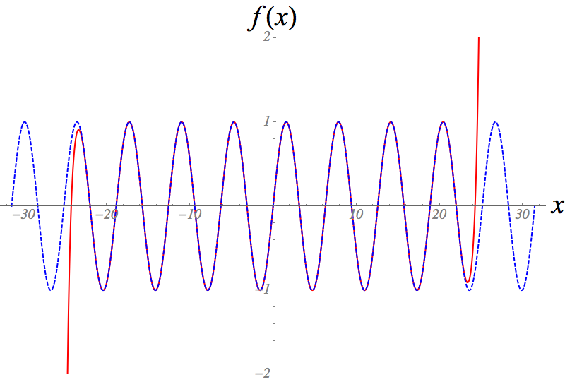
To illustrate how the Taylor polynomials around \(x=0\) approximate \(\sin x\), here is an image showing the Taylor polynomial of degree \(61\) for \(\sin x\) (the red curve), together with \(\sin x\) itself (the blue dashed curve).
Similarly, it can be shown that the following functions equal their Taylor series expansions: \[\begin{aligned} \cos x &= \sum_{k=0}^\infty \frac{(-1)^k x^{2k}}{(2k)!} \qquad \text{ for all } x \in \mathbb{R}, \\[1mm] \log(1+x) &= \sum_{k=1}^\infty \frac{(-1)^{k+1} x^{k}}{k} \qquad \text{ for all } x \in \mathbb{R} \text{ with } |x| < 1, \\[1mm] \frac{1}{1-x} &= \sum_{k=0}^\infty x^k \qquad \text{ for all } x \in \mathbb{R} \text{ with } |x| < 1. \end{aligned}\] In the latter two cases, the radius of convergence of the Taylor series is \(1\) (think about what happens if you choose a particular \(x \in \{\pm 1\}\), i.e. \(|x| = 1\), in each case), which coincides with the fact that the functions themselves are undefined for certain values of \(x\).
Critical points in 1 dimension
A “critical point” is the generic name for an extreme point in the system.
A critical point \(a\) can be of one of three types:
a (local) minimum (and stable) if \(f(x) > f(a)\) for all \(x\) near \(a\) (\(x \neq a\));
a (local) maximum (and unstable) if \(f(x) < f(a)\) for all \(x\) near \(a\) (\(x \neq a\));
an inflection point, if it is neither a (local) maximum nor a (local) minimum.
We can use the Taylor polynomial/series to help determine which types of critical point we have.
Before doing this, perhaps it is helpful to indicate where the terminology “stable” and “unstable” comes from – this is from physics.
In general, if \(f(x)\) has a critical point at \(x=a\), then we have \[f(x)\approx f(a)+\,\frac{f''(a)}{2}(x-a)^2,\] and we conclude that \(x=a\) is a local maximum if \(f''(a)<0\) (even if we cannot be bothered to plot \(f\)), and that \(x = a\) is a local minimum if \(f''(a)>0\). Therefore, we can discover and classify the critical points of a differentiable function \(f(x)\) as follows.
Find all points \(a\) where \(f'(a)=0\).
Find the numerical value of \(P=f''(a)\).
If \(P<0\) it is a maximum, if \(P>0\) it is a minimum. If \(P=0\) we cannot conclude what type of critical point it is, and we need more information.
An example where \(P=0\) occurs at the cricial point \(x=0\) of the function \(f(x) = x^{4}\). Although \(f(x) = x^4\) has a minimum at \(x = 0\), we have \(P = f''(0) = 0\). On the other hand, \(x=0\) is also a critical point of the function \(g(x) = x^{3}\) and, again, \(P = g''(0) = 0\), but in this case \(g(x)\) has an inflection point at \(x=0\).
Back to SMB Term 2.…
3.2.1 Multivariate Taylor expansions
Let me first slightly rephrase the Taylor series as a function of \(h\), the displacement from \(x=a\): \[f(a+h)=f(a)+hf'(a)+\frac{h^{2}}{2!}f''(a)+\ldots\] We can also write it as an operator equation using the fact that, as we just saw, \(e^{A}=1+A+\frac{A^{2}}{2!}+\ldots\) \[f(a+h)=e^{h\odv{}{x}}f(x)|_{x=a}\,\,\,.\] This last equation makes it obvious how to generalise: a function of two variables expanded about \((x,y)=(a,b)\) can be found by first expanding about \(x=a\) and then about \(y=b\); doing this explicitly we first get \[f(a+h,b+k)=f(a,b+k)+hf_{x}(a,b+k)+\frac{h^{2}}{2!}f_{xx}(a,b+k)+\ldots\] Next we approximate \(f(a,b+k)\) and the derivatives in \(x\), by in turn expanding them as Taylor series in \(y\) about \(y=b\). That is \[\begin{aligned} f(a,b+k) & =f(a,b)+kf_{y}(a,b)+\frac{k^{2}}{2!}f_{yy}(a,b)\ldots\nonumber \\ f_{x}(a,b+k) & =f_{x}(a,b)+kf_{xy}(a,b)+\ldots\nonumber \\ f_{xx}(a,b+k) & =f_{xx}(a,b)+kf_{xxy}(a,b)+\ldots \end{aligned}\]
Keeping terms up to quadratics (obviously we can extend but it gets a bit laborious) we have:
I now present an alternative way to arrive at this formula, which may or may not help you in understanding it. This form uses the operator understanding of the Taylor expansion. That is \[\begin{aligned} f(a+h,b+k) & = e^{h\partial_{x}}e^{k\partial_{y}}f(x,y)|_{x=a,y=b}\nonumber \\ & = e^{h\partial_{x}+k\partial_{y}}f(x,y)|_{x=a,y=b}\nonumber \\ & = \left(1+h\partial_{x}+k\partial_{y}+\frac{1}{2}(h\partial_{x}+k\partial_{y})^{2}+\ldots\right)f(x,y)|_{x=a,y=b}\nonumber \\ & = f+hf_{x}+kf_{y}+\frac{1}{2}(h^{2}f_{xx}+2hkf_{xy}+k^{2}f_{yy})+...\label{eq:Taylor2} \end{aligned}\] Note that we have arrived at the same result. This approach is powerful but we will not use it too much in these lectures. As an aside, it is worth mentioning that the reason that we can combine the exponentials trivially, \(e^{h\partial_{x}}e^{k\partial_{y}}\equiv e^{h\partial_{x}+k\partial_{y}}\), is that the operators in the exponent “commute”, by which we mean that it doesn’t matter which way round they go, namely \(\partial_{x}\partial_{y}=\partial_{y}\partial_{x}\). This is thanks to Clairault’s theorem again.
Note that in a space of variables \(\mathbf{x}=(x_{1},\dots, x_{n})\) we can write the expansion of \(f\) at \(\mathbf{x}=\mathbf{x_{0}}+\mathbf{h}\) as \[f(\mathbf{x_{0}+h})=e^{\mathbf{h}.\nabla}f|_{\mathbf{x_{0}}}\,\,.\label{eq:TaylorN}\]
Suggested questions: Q10-12.
3.3 Critical points
Recap of 1-dimensional case
The critical points of a function \(f:\mathbb{R}\rightarrow\mathbb{R}\) are all the points with \(f_{x}=0\). If \(f_{xx}>0\) it is a local minimum. If \(f_{xx}<0\) it is a local maximum. If \(f_{xx}=0\) (e.g. \(f=x^{4}\) at \(x=0\)) more analysis is needed.
3.3.1 2-dimensional case
We wish to generalise this to find critical points, and say whether they are local maxima, minima, or saddle-points in 2 or more dimensions. A critical point is a point at which both \(f_{x}=0\) and \(f_{y}=0\). Or equivalently, \(\nabla f=\mathbf{0}.\)
Distinguishing local maxima and minima using the Taylor expansion:
Let us now be somewhat more formal.
We can use the Taylor expansion about \((a,b)\) to tell us about the nature of the point there. To simplify things call \(h=x-a\) and \(k=y-b\) and call \[\begin{aligned} P & = f_{xx}(a,b)\\ Q & = f_{xy}(a,b)\\ R & = f_{yy}(a,b). \end{aligned}\] Then using the Taylor expansion, we can write \[f(x,y)=f(a,b)+hf_{x}(a,b)+kf_{y}(a,b)+\frac{1}{2}(h^{2}P+2hkQ+k^{2}R)+\ldots\] A necessary condition for a local maximum, local minimum or saddle point is that \(f_{x}=f_{y}=0\).
The test for what sort of critical point it is:
Proof: From the Taylor expansion, the value of the function near \((a,b)\) can be approximated by a quadratic polynomial (whose linear term vanishes because \((a,b)\) is a critical point): \[\begin{aligned} f(a+h, b+k) &\approx f(a,b) + \frac{1}{2P}(h^{2}P^{2} + 2hkQP + k^{2}RP) \\ &= f(a,b) + \frac{1}{2P}((hP+kQ)^{2}+k^{2}M). \end{aligned}\] If \(P>0\) and \(M>0\) then \(f(a+h, b+k)-f(a,b)>0\) and \(f(a,b)\) is a minimum. If \(P<0\) then the reverse is true. If \(M<0\) then for some values of \(h,k\) \(f(a+h, b+k)-f(a,b)\) is positive and for others it’s negative; thus we have a saddle point.
3.3.2 \(n\)-dimensional case
Not examined: just for completeness.
We can generalise this to any number of dimensions. Let \(f:\mathbb{R}^{n}\rightarrow\mathbb{R}\). Critical points are given by \(\nabla f(a)=\mathbf{0}.\) To determine their nature, define the Hessian: \[H_{ij}\,=\,\pdv{f}{x_i,x_j}\,\,.\] The Taylor expansion in \(n\) dimensions near that point \(\mathbf{x} = \mathbf{a}\) is given by the following expression, which is a generalization to multiple variables of Equation 3.4: \[f(\mathbf{x}) = \sum_{i=1}^{n} (x_i - a_i) \pdv{f}{x^i}(\mathbf{a}) + \frac{1}{2} \sum_{i,j=1}^{n} H_{ij}(\mathbf{a}) (x_i - a_i)(x_j-a_j)\] At a critical point the first term vanishes. So to figure out what happens we need to understand the term with the \(H_{ij}\). We now need to know a little bit of linear algebra – consider the \(n\) eigenvalues of \(H_{ij}\). If they are all positive (i.e. \(H_{ij}\) is positive definite) then it is a local minimum. All negative (i.e. \(H_{ij}\) is negative definite) it is a maximum. If there are both positive and negative eigenvalues it is a saddle. Note that in two dimensions we have \(H_{ij}=\left(\begin{array}{cc} P & Q\\ Q & R \end{array}\right)\), and positive or negative definiteness is guaranteed by \(M=\det H>0\), giving precisely the criteria specified above.
Suggested questions: Q8, Q13.
...but why don’t you like matrices?↩︎