$$ \usepackage{derivative} \newcommand{\odif}[1]{\mathrm{d}#1} \newcommand{\odv}[2]{\frac{ \mathrm{d}#1}{\mathrm{d}#2}} \newcommand{\pdv}[2]{\frac{ \partial#1}{\partial#2}} \newcommand{\th}{\theta} \newcommand{\p}{\partial} \newcommand{\var}[1]{\text{Var}\left(#1\right)} \newcommand{\sd}[1]{\sigma\left(#1\right)} \newcommand{\cov}[1]{\text{Cov}\left(#1\right)} \newcommand{\cexpec}[2]{\mathbb{E}\left[#1 \vert#2 \right]} $$
6 Integrating Functions of Several Variables
Up till now we have considered integrals of functions of one variable, such as \[\int_{0}^{2} x^2 \odif{x}.\] We will now begin to study integrals in multiple variables. Before getting into the formalities, let’s begin with an example.
We can even allow the limits on the first integration (with respect to \(y\) in this case) to depend on the other variable (in this case, \(x\)), so that we can integrate over more complicated regions in \(\mathbb{R}^2\).
What we have just done is the basic idea of integration in multiple dimensions! But what does it mean?
6.1 Interpretation as volume under a surface
Recap of the one-dimensional (Riemann) integration
Recall that the area under a curve \(f(x)\) between \(x=a\) and \(x=b\) is given by \[S=\int_{a}^{b}f(x)\odif{x}.\] To approximate this area, we partition the interval \([a,b]\) into \(N\) subintervals of length \(\delta x_{1},\delta x_{2}, \ldots, \delta x_{N}\), respectively, and let \(x_{i}\) be the point midway along the \(i^\text{th}\) subinterval. Then the area is approximately given by the sum of the area of all the rectangles of height \(f(x_{i})\) and width \(\delta x_{i}\): \[S\approx\sum_{i=1}^{N}f(x_{i}) \, \delta x_{i}.\] To find the integral we take the limit as \(N\rightarrow\infty\) \[S=\lim_{N\rightarrow\infty}\left(\sum_{i=1}^{N}f(x_{i}) \, \delta x_{i}\right) =\int_{a}^{b}f(x)\odif{x}.\]
Extension to two-dimensional (Riemann) integration
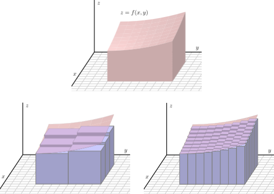
Suppose we want to calculate the volume under a surface whose height is given by \(f(x,y)\). Let the region in the \(xy\)-plane that we want to integrate over be \(R\) so that we might guess that \[V=\iint_{R}f(x,y)\,\odif{A}.\] To see that this is indeed the volume, approximate the volume by dividing the integration region into \(N\) subregions of area \(\delta A_{1},\delta A_{2}\ldots\delta A_{N}\), respectively. Let \((x_{i},y_{i})\) be the point “in the middle” of the \(i^\text{th}\) subregion. Then the volume is approximately given by the sum of the volumes of all the columns of height \(f(x_{i},y_{i})\) and base area \(\delta A_{i}\): \[V\approx\sum_{i=1}^{N}f(x_{i},y_{i}) \, \delta A_{i}.\] The double integral is defined as the limit of this sum as \(N\rightarrow\infty\); that is, so that \[\begin{aligned} V = \lim_{N\rightarrow\infty}\left(\sum_{i=1}^{N}f(x_{i},y_{i}) \, \delta A_{i} \right) = \iint _{R}f(x,y)\,\odif{A}. \end{aligned}\]
6.1.1 Integration over rectangular regions
So far, so formal. How do we see that the limit above is the same thing as the earlier double integrations?
Consider the rectangular region \(R\) from a previous example that was given by \(0\leq x\leq1\) and \(0\leq y\leq2\). We’d like to integrate a function \(f(x,y)\) over this rectangular region \(R\) (as in the previous example) and we claim that this double integral should give the volume under the surface of height \(z = f(x,y)\). Let’s investigate why this is the case.
We can partition the rectangular region \(R\) into \(N=mn\) sub-rectangles by partitioning the interval \(0 \leq x \leq 1\) into \(m\) subintervals of length \(\delta x_{1},\delta x_{2}, \ldots, \delta x_{m}\), respectively, and the interval \(0 \leq y \leq 2\) into \(n\) subintervals of length \(\delta y_{1},\delta y_{2}, \ldots, \delta y_{n}\), respectively. Then there are \(N=mn\) sub-rectangles indexed by pairs \((i,j)\) (i.e. the \(i^\text{th}\) \(x\)-subinterval and the \(j^\text{th}\) \(y\)-subinterval combine to give the \((i,j)^\text{th}\) sub-rectangle), and the area of the \((i,j)^\text{th}\) sub-rectangle is \(\delta A_{ij} = \delta x_i \delta y_j\).
Then the volume under the surface \(z = f(x,y)\) over the rectangular region \(R\) is approximated by the double sum \[V \approx \sum_{i=1}^{m} \left( \sum_{j=1}^n f(x_{i},y_{j}) \, \delta y_{j} \right) \delta x_i \,,\] where \((x_i, y_j)\) is some chosen of point in the \((i,j)^\text{th}\) sub-rectangle and where we sum over the \(y\)-direction first only to ensure that our final double integration will do the \(y\)-integration first. As before, the idea is to take the limit of each summation as \(m\) and \(n\) go to infinity and, hence, to obtain \[V = \lim_{m \to \infty} \sum_{i=1}^{m} \left( \lim_{n \to \infty} \sum_{j=1}^n f(x_{i},y_{j}) \, \delta y_{j} \right) \delta x_i = \int_0^1 \int_0^2 f(x,y) \, \odif{y} \odif{x} \,.\]
Another way to think of this is that, for each \(x_i\), we compute the area under the curve \(f(x_{i},y)\) at \(x=x_{i}\), which is given by the single integration limit \[\begin{aligned} A(x_{i}) = \lim_{n\rightarrow\infty}\sum_{j = 1}^{n} f(x_{i},y_{j}) \, \delta y_{j} = \int_{0}^{2} f(x_{i},y) \, \odif{y}\,. \end{aligned}\] Since \(x_i\) lies in a subinterval of thickness \(\delta x_i\), we obtain a slice of volume \(A(x_i) \, \delta x_i\) of our desired total volume, and we add up (via the index \(i\)) the volumes of all \(m\) such slices. Now taking the limit of this sum as \(m\) goes to infinity, we obtain \[\begin{aligned} V &= \lim_{m \rightarrow\infty}\sum_{i=1}^{m}A(x_{i}) \, \delta x_{i} \\ &= \int_{0}^{1} A(x) \, \odif{x}\\ &= \int_{0}^{1}\int_{0}^{2}f(x,y) \, \odif{y}\odif{x} \,. \end{aligned}\] Note that, in this particular case, we can do the integration in either order (by swapping the roles of \(x\) and \(y\) in the argument above). For double integrals over more complicated areas (i.e. not rectangles), you have to be careful with the limits.
An important example of double integration over a region \(R\) is when we have the constant function \(f(x,y) \equiv 1\). In this case, the “volume” under this surface is clearly just the area of the region of integration \(R\); that is, \[\iint_{R}\odif{A}= \text{Area}(R).\]
6.2 Double integrals and limits of integration
Most regions of integration \(R\) of interest to us could, perhaps, be described most naturally in a coordinate system (e.g. polar) other than the Cartesian coordinate system \((x,y)\). Nevertheless, we can often still describe the region \(R\) in Cartesian coordinates. With this in mind, suppose that the region \(R\) is described by the limits \[ a \leq x \leq b \quad \text{ and } \quad u(x) \leq y \leq v(x), \tag{6.1}\] where \(u(x)\) and \(v(x)\) are some functions of \(x\). This is saying that, as \(x\) varies between \(x=a\) and \(x=b\), the region \(R\) is bounded above by the curve \(y=v(x)\) and below by the curve \(y=u(x)\). Integration over the region \(R\) then becomes \[\iint_{R}f(x,y) \, \odif{A}=\int_{a}^{b}\int_{u(x)}^{v(x)}f(x,y) \, \odif{y}\odif{x}.\] Note that the interpretation as the limit of sums is unchanged from earlier, but that now we cannot just blindly switch the order of integration, because the internal limits are explicitly dependent on the variable \(x\).
If we wish to change the order of integration, we need to (carefully) rewrite the limits appearing in Equation 6.1 so that they’re of the form \[c \leq y \leq d \quad \text{ and } \quad r(y) \leq x \leq s(y),\] for some functions \(r(y)\) and \(s(y)\) of \(y\). We can do this either algebraically or, often much easier, by drawing out the region of integration and reading off the limits.
Recall that the area of a region \(R\) in the \(xy\)-plane is given by \[\text{Area}(R) = \iint_{R}\odif{A}.\]
6.2.1 Making difficult integrals easier by changing the order of integration
Sometimes it is difficult to evaluate double integrals in the form in which they first appear, but switching the order of integration results in a much easier computation. However, as always, we need to be very careful with the limits.
Let’s return to probability for a moment. Recall from Equation 1.1 in (ch-prob?) that we can compute the probability that continuous random variables \(X\) and \(Y\) take values in a region \(R\) of the \(xy\)-plane by evaluating a double integral of their joint probability density function \(f_{X,Y}\) over the region \(R\). We now have the machinery to elaborate upon this.
6.2.2 Integration in polar coordinates
For some double integrals, where the region of integration displays rotational symmetry, it is easier to use polar coordinates. We cover the \(xy\)-plane with a polar grid and our area elements \(\delta A\) become wedges at \((r,\theta)\) as shown below:
Note that for the Cartesian coordinate system \((x,y)\) we had \[\odif{A} = \odif{x} \odif{y}\] and we need to modify this for polar coordinates. It is not as simple as swapping \(x\) and \(y\) with \(r\) and \(\theta\), however. We need to understand the area elements of the wedges mentioned above (which are not quite rectangular): the area of such a wedge of length \(\delta{r}\) and width \(r \delta \theta\) is given by \(\delta{A}=r \delta{r} \delta \theta\). Thus, when we are integrating with respect to polar coordinates we have \[\odif A = r \, \odif r \odif \theta.\] Moreover, the function \(f(x,y)\) to be integrated also needs to be rewritten in terms of polar coordinates using \(x = r \cos \theta\), \(y = r \sin \theta\); that is, \(f(x,y)\) becomes \(f(r\cos\theta,r\sin\theta)\). Therefore, we get the “theorem”
It is crucial to note that what we have just seen is that the “integration measure” – i.e. the \(\odif{A}\) at the end – is different in different coordinates. We will derive a general formula for this later on, but for now let’s look at some examples.
The following example is a famous and clever use of double integrals to evaluate a difficult integral in one variable.
6.3 Triple integrals
Many problems require the evaluation of a “bulk” property, such as the mass of a three-dimensional object, by integrating over the entire volume. For example, suppose we want to find the mass of a star of density \(\rho(x,y,z)\). Recall that mass is given by volume times density. Thus, the mass \(\delta M\) of a small region with volume \(\delta V\) (e.g. a small cube with sides \(\delta {x}\), \(\delta {y}\), \(\delta z\)) and density \(\rho(x,y,z)\) will be \[\delta M = \rho(x,y,z) \, \delta V.\] Now, given a three-dimensional object \(R \subseteq \mathbb R^3\) of density \(\rho(x,y,z)\), we can subdivide \(R\) into \(N\) small subregions, compute the mass \(\delta M_i\) of each subregion, and then approximate the total mass \(M\) of \(R\) by adding up the masses \(\delta M_i\). Letting \(N\) tend to infinity, we find that the total mass of \(R\) can be written as as the triple integral \[M = \iiint_{R}\rho(x,y,z) \, \odif{V} = \iiint_{R}\rho(x,y,z) \, \odif{x}\odif{y}\odif{z}.\] Moreover, if the density function is the constant function \(\rho(x,y,z) \equiv 1\), observe that the volume of the (three-dimensional) region is given by \[\mathrm{Vol}(R) = \iiint_R \, \odif V.\]
6.3.1 Cylindrical polar coordinates
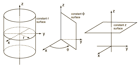
As with double integration, there are often cases where different coordinate systems are preferable. Cylindrical polar coordinates are useful in cases with axial symmetry, usually involving pipes, cylinders, annuli, and so on. They are an extension to two-dimensional polar coordinates, where we essentially just “add a \(z-\)coordinate”. To tie in with convention, we’ll now call the angular coordinate \(\phi\), rather than \(\theta\), although in practice you can use whichever symbol you like. The description of an arbitrary point \((x,y,z)\) in terms of cylindrical polar coordinates \((r,\phi, z)\) is illustrated in the figure, as is how to visualise the surfaces obtained by taking one of the coordinates \((r,\phi, z)\) to be constant.
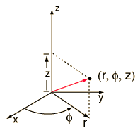
We describe \((x,y,z)\) in terms of \((r, \phi, z)\) by extending the coordinate transformation for (planar) polar coordinates; that is, \[x = r \cos \phi, \qquad y = r \sin \phi , \qquad z = z.\] To write the volume element \(\odif V\) in terms of the cylindrical polar coordinates \((r,\phi, z)\), we extend the ideas from the case of (planar) polar coordinates into three dimensions (i.e. we find the volume of a small, approximately cubular region of sidelengths \(\delta {r}\), \(r \delta {\phi}\) and \(\delta {z}\)) to obtain \[\odif V = r \, \odif r \odif \phi \odif z\] and, hence, \[\iiint_{R}f(x,y,z) \, \odif V = \iiint_{R}f(x,y,z) \,\odif{x}\odif{y}\odif{z} = \iiint_{R}f(r\cos\phi,r\sin\phi,z)\,r\odif{r}\odif{\phi} \odif{z}.\]
6.3.2 Spherical polar coordinates
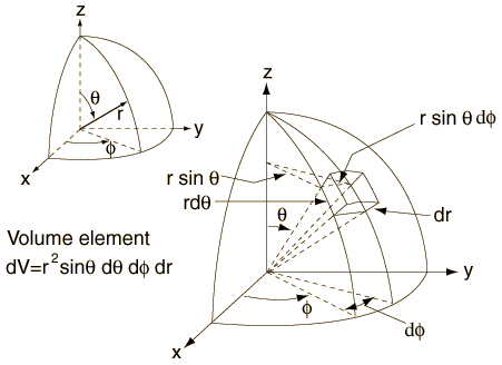
Spherical polar coordinates are useful in cases with radial symmetry: for example, cases involving central charges, gravitating stars, black holes, bubbles, explosions, etc. In spherical polar coordinates, a point \((x,y,z) \in \mathbb R^3\) is described by the radius \(r = \sqrt{x^2 + y^2 + z^2}\) (the distance from the origin) and two angles, one altidudinal angle \(\theta \in [0, \pi]\) measured from the positive \(z\)-axis (essentially giving “latitude”) and one “azimuthal” angle \(\phi \in [0, 2\pi)\) measured in the \(xy\)-plane from the positive \(x\)-axis (essentially giving “longitude”), as illustrated in the diagram below.
It is important to remark that the \(r\) appearing in spherical polar coordinates (in this section) is not the same as the \(r\) appearing in cylindrical polar coordinates (in the last section).
Observe that the given ranges of values for the coordinates \(r\), \(\theta\) and \(\phi\) allow for points \((0,0,z) \in \mathbb R^3\) along the \(z\)-axis to have multiple representations in spherical polar coordinates: for example, the origin \((x,y,z) = (0,0,0)\) is given by \((0,\theta, \phi)\), where \(\theta \in [0, \pi]\) and \(\phi \in [0, 2\pi)\) are arbitrary, while the point \((0,0,z)\) is given in spherical polar coordinates by \((z,0, \phi)\), if \(z > 0\), and by \((-z, \pi, \phi)\), if \(z < 0\), with \(\phi \in [0, 2\pi)\) arbitrary in each case. Thus, if we want our spherical polar coordinate system to give a unique description of every point in \(\mathbb R^3\), then we need to decide upon a convention for points along the \(z\)-axis (e.g. we could agree to always describe the origin as \((r, \theta, \phi) = (0,0,0)\) and other points on the \(z\)-axis by \((r, \theta, \phi) = (z, 0, 0)\), if \(z > 0\), or by \((r, \theta, \phi) = (-z, \pi, 0)\), if \(z < 0\)). However, in practice, we typically ignore these issues with points along the \(z\)-axis when doing integration, as they don’t have any impact on the outcome.
Some elementary trigonometry yields that the coordinates \((x,y,z)\) can be written in terms of the spherical polar coordinates \((r, \theta, \phi)\) via the coordinate transformation \[ x = r \sin \theta \cos \phi, \quad y = r \sin \theta \sin \phi, \quad z = r \cos \theta. \tag{6.2}\] To write the volume element \(\odif V\) in terms of the spherical polar coordinates \((r,, \theta, \phi)\), we again extend the ideas from the case of (planar) polar coordinates into three dimensions (i.e. we find the volume of a small, approximately cubular region of sidelengths \(\delta {r}\), \(r \delta \theta\) and \(r \sin \theta \delta \phi\)) to obtain \[\odif V = r^2 \sin \theta \, \odif r \odif \theta \odif \phi\] and, hence, \[\iiint_{R}f(x,y,z) \, \odif V = \iiint_{R} f(r\sin\theta\cos\phi,r\sin\theta\sin\phi,z\cos\theta)\,r^{2} \sin\theta \, \odif{r} \odif{\theta} \odif{\phi}.\]
6.4 The Jacobian
We have seen that whenever we perform a change of coordinates in order to compute an integral, we pay the price of introducing an additional factor in the integrand. Up to now, we have determined this additional factor by drawing an ad-hoc diagram of a small region determined by a small change in each of the new coordinates and computing its area or volume. There is a simple and important general formula for this additional factor which avoids the need to test our artistic skills. To understand it, suppose first that we are doing an integral over one variable: \[\begin{aligned} \int f(x) \odif{x}. \end{aligned}\] Now imagine we want to change our variable \(x\) into a variable \(u = u(x)\) (similarly to doing an integration by substitution). How does the integral change? We can re-express the function \(f(x)\) in terms of the variable \(u\) as \(f(x(u))\) (by inverting \(u=u(x)\) to find \(x\) in terms of \(u\), i.e. \(x = x(u)\)), but we also need to introduce an additional factor, so that \[\int f(x) \odif{x} = \int f(x(u)) \, \odv{x}{u} \, \odif{u}.\] That is, we transformed the variable from \(x\) to \(u\), at the cost of picking up an extra factor of \(\odv{x}{u}\). As we know from doing integration by substitution, we can write \[ \odif{x} = \odv{x}{u} \, \odif{u} \quad \text{ and } \quad \odif{u} = \odv{u}{x} \odif{x}. \tag{6.3}\]
Now, as usual, we care about the \(n\)-dimensional version of this. Suppose that we need to evaluate an \(n\)-dimensional integral \[\iint...\int f(x_{1},..x_{n}) \, \odif{x_{1}}...\odif{x_{n}}\] and that we can do this by transforming to a new coordinate system \((u_1, u_2, \dots, u_n)\). The old coordinates \((x_1, x_2, \dots, x_n)\) can be written in terms of the new ones (like we did for the various instances of polar coordinates we discussed), so that \[x_j = x_j(u_1, u_2, \dots, u_n),\] for all \(j \in \{1, 2, \dots, n\}\). Then we can write the multiple-dimensional analogue of Equation 6.3 is expressed as \[\odif{x_1} \odif{x_2} \dots \odif{x_n} = | J(u_1, u_2, \dots, u_n) | \, \odif{u_1} \odif{u_2} \dots \odif{u_n},\] where \(| J(u_1, u_2, \dots, u_n) |\) is the absolute value of the determinant \[J(u_1, u_2, \dots, u_n) = \det \begin{pmatrix} \pdv{x_1}{u_1} & \pdv{x_1}{u_2} & \cdots & \pdv{x_1}{u_n} \\ \pdv{x_2}{u_1} & \pdv{x_2}{u_2} & \cdots & \pdv{x_2}{u_n} \\ \vdots & \vdots & \ddots & \vdots\\ \pdv{x_n}{u_1} & \pdv{x_n}{u_2} & \cdots & \pdv{x_n}{u_n} \end{pmatrix} \] The function \(J(u_1, u_2, \dots, u_2)\) is called the Jacobian and the matrix of partial derivatives is called the Jacobian matrix.
As an example, consider the transformation to polar coordinates in two dimensions. Here we have \(x=r\cos\theta\) and \(y=r\sin\theta\), so that \[\begin{aligned} J(r, \theta) &= \det \begin{pmatrix} \pdv{x}{r} & \pdv{x}{\theta} \\ \pdv{y}{r} & \pdv{y}{\theta} \end{pmatrix} \\ &=\det \begin{pmatrix} \cos\theta & -r\sin\theta\\ \sin\theta & r\cos\theta \end{pmatrix} = r. \end{aligned}\] Hence, we obtain \(\odif{x}\odif{y}= | J(r, \theta) | \, \odif{r}\odif{\theta}= r \, \odif{r}\odif{\theta}\), in agreement with the area element previously computed using pictures.
As a further example, consider the transformation to spherical polar coordinates in three dimensions. From the expressions in Equation 6.2, we have \[\begin{aligned} J(r, \theta, \phi) & =\det \begin{pmatrix} \pdv{x}{r} & \pdv{x}{\theta} & \pdv{x}{\phi} \\ \pdv{y}{r} & \pdv{y}{\theta} & \pdv{y}{\phi} \\ \pdv{z}{r} & \pdv{z}{\theta} & \pdv{z}{\phi} \\ \end{pmatrix} \\ &=\det \begin{pmatrix} \sin\theta\cos\phi & r\cos\theta\cos\phi & -r\sin\theta\sin\phi\\ \sin\theta\sin\phi & r\cos\theta\sin\phi & r\sin\theta\cos\phi\\ \cos\theta & -r\sin\theta & 0 \end{pmatrix} \\ &= \cos\theta(r^{2}[\cos^{2}\phi+\sin^{2}\phi]\,\cos\theta\sin\theta)+r^{2}\sin^{3}\theta[\cos^{2}\phi+\sin^{2}\phi]\\ &= r^{2}\cos^{2}\theta\sin\theta+r^{2}\sin^{3}\theta\\ &= r^{2} \sin \theta. \end{aligned}\] Therefore, since \(\sin \theta \geq 0\) for all \(\theta \in [0, \pi]\), we have \[\odif{x}\odif{y}\odif{z} = | J(r, \theta, \phi) | \, \odif{r} \odif{\theta} \odif{\phi} = r^{2} \sin \theta \, \odif{r} \odif{\theta} \odif{\phi},\] exactly the same volume element that we found by considering a picture of the small region obtained by small changes in each of the coordinates.
6.5 Applications: Centre of Mass, centroids and moments of inertia
The centroid of a body is its average coordinate.
That is, it is the point with coordinates \[ \bar{x}=\frac{\iiint x\,\odif{V}}{\iiint\,\odif{V}}, \qquad \qquad \bar{y}=\frac{\iiint y\,\odif{V}}{\iiint\,\odif{V}}, \qquad \qquad \bar{z}=\frac{\iiint z\,\odif{V}}{\iiint\,\odif{V}}. \]
To simplify things, we sometimes write all three coordinates in terms of \(\bar{x} = (x,y,z)\): \[\bar{\mathbf{x}}=\frac{\iiint\mathbf{x}\,\odif{V}}{\iiint\,\odif{V}}.\]
The centre of mass of a body is its average coordinate weighted by the mass density. That is, if the density as a function of position \(\mathbf{x}\) is \(\rho(\mathbf{x})\), then \[\bar{\mathbf{x}}=\frac{\iiint\mathbf{x}\rho(\mathbf{x})\,\odif{V}}{\iiint\rho(\mathbf{x})\,\odif{V}}.\]
The moment of inertia of a body is the average squared distance of a body from an axis of rotation, weighted by the mass density: \[I=\iiint r(\mathbf{x})^{2}\rho(\mathbf{x})\,\odif{V},\] where \(r(\mathbf{x})\) is the perpendicular distance of the point \(\mathbf{x}\) from the axis of rotation.