5  Vector Calculus of Vector Fields

5.1 Vector fields

So far our focus has been almost entirely on scalar functions. These are real-valued functions \(f:\mathbb{R}^{n}\rightarrow\mathbb{R}\) which associate a single number \(f(x_1, x_2, \dots, x_n)\) with each coordinate point \((x_1, x_2, \dots, x_n)\in \mathbb{R}^n\) (e.g. the temperature as a function of location).

However, we may need to do more: often we need to describe quantities that have vector properties at each coordinate point. An example might be the wind: this points in a direction and has a magnitude at each coordinate point. If we ignore height for a second, then the wind map is clearly a function from a region in \(\mathbb{R}^2\) (i.e. a region on the surface of the earth) to \(\mathbb{R}^2\), i.e. the space of two-dimensional vectors.

From physics, we also have the examples of the electric field \(\mathbf{E}\) and the magnetic field \(\mathbf{B}\), which are both functions of the variables \(x,y,z\) (and also \(t\)) that themselves have three vector components.

So we now define:

🔑 Key idea

A vector field is a function \(\boldsymbol{V} \colon \mathbb{R}^n \to \mathbb{R}^n\) which assigns a vector \(\boldsymbol{V}(\mathbf{x}) = \boldsymbol{V}(x_1, x_2, \dots, x_n)\) in \(\mathbb{R}^n\) to each point \(\mathbf{x} = (x_1, x_2, \dots, x_n) \in \mathbb{R}^n\).

For example, a vector function \(\boldsymbol{V}\) between \(\mathbb{R}^3\) and \(\mathbb{R}^3\) (usually written \(\boldsymbol{V} \colon \mathbb{R}^3 \to \mathbb{R}^3\)) would take the form \[\boldsymbol{V}(x,y,z)=V_{1}(x,y,z)\boldsymbol{i}+V_{2}(x,y,z)\boldsymbol{j}+V_{3}(x,y,z)\boldsymbol{k}.\] It’s also quite common when writing vector fields to use the coordinates themselves as indices for the coordinate functions, rather than numbers, e.g. \[\boldsymbol{V}(x,y,z)=V_{x}(x,y,z)\boldsymbol{i}+V_{y}(x,y,z)\boldsymbol{j}+V_{z}(x,y,z)\boldsymbol{k}.\] However, this latter notation clashes with our subscript notation for partial derivatives and would lead to unnecessary confusion. Therefore, in this module we will stick to the first notation (with indices given by numbers).

We have already seen an explicit example of a vector field, although we didn’t dwell on this fact at the time; namely, if \(f(x_1, x_2, \dots, x_n)\) is a (scalar) function, then its gradient \(\boldsymbol{\nabla}f = \left( \pdv{f}{x_1}, \pdv{f}{x_2}, \dots, \pdv{f}{x_n} \right)\) is a vector field \(\boldsymbol{\nabla}f \colon \mathbb{R}^n \to \mathbb{R}^n\).

💪 Try it out

When \(\boldsymbol{V}: \mathbb{R}^2 \to \mathbb{R}^2\), we can sketch out the vector function by drawing an arrow at each point.

Figure 5.1: Examples of vector fields: \(\boldsymbol{V}=x\boldsymbol{i}+y\boldsymbol{j}\) on the left and \(\boldsymbol{V}=-y\boldsymbol{i}+x\boldsymbol{j}\) on the right. The magnitude of the arrows is \(\sqrt{V_{1}^{2}+V_{2}^{2}}=r\) in both of these cases.

How do we differentiate a vector field? You should note that there is basically now a matrix worth of information from differentiating each component with respect to each argument, i.e. \(\p_{x} V_{x}, \p_{y} V_{y}\) etc. It turns out there are some important ways to arrange this information.

So first, like the scalar functions we may define:

🔑 Key idea

The total derivative of a vector-valued function \(\boldsymbol{V}\) is the vector \[\odif{\boldsymbol{V}}=\pdv{\boldsymbol{V}}{x} \odif{x} +\pdv{\boldsymbol{V}}{ y}\odif{y}+\pdv{\boldsymbol{V}}{z} \odif{z}.\]

💪 Try it out

If \(\boldsymbol{V}=(2x^{2}y,\sin(xy),y^{3}ze^{z})\), then

\[\begin{aligned} \pdv{\boldsymbol{V}}{x}&=(4xy,x\cos xy,0), \\ \pdv{\boldsymbol{V}}{y}&=(2x^2,y\cos xy,3y^2 ze^z), \\ \pdv{\boldsymbol{V}}{z}&=(0,0,y^3(z^2+1) e^z), \end{aligned}\] so \[\begin{aligned} \odif{\boldsymbol{V}} = \left( 4xy \odif{x} + 2x^2 \odif{y}, \cos(xy) (x \odif{x} + y \odif{y}), e^z( 3y^2 z \odif{y} + y^3 (z^2+1) \odif{z}) \right). \end{aligned}\]

We also have the chain rule for vector-valued functions:

🔑 Key idea

For a function \(\boldsymbol{V}(x,y,z)\), considered at the point \(\mathbf{x}(t) = (x(t), y(t), z(t))\), we have \[\begin{aligned} \frac{d\boldsymbol{V}}{dt} & =\pdv{\boldsymbol{V}}{x}\odv{x}{t} + \pdv{\boldsymbol{V}}{y} \odv{y}{t} + \pdv{\boldsymbol{V}}{z} \odv{z}{t} \\ & \equiv\left(\frac{\mathrm{d}\mathbf{x}}{dt}\cdot\boldsymbol{\nabla}\right)\boldsymbol{V}. \end{aligned}\]

We now introduce two new notions of derivative, i.e., ways to capture the information present in these vector fields: they are called divergence and curl.

5.2 Divergence

Recall that, when dealing with situations involving \(n\) variables \(x_1, x_2, \dots, x_n\), we introduced the differential operator \[\boldsymbol{\nabla} = \left(\pdv{}{x_1}, \pdv{}{x_2}, \dots, \pdv{}{x_n}\right).\]

🔑 Key idea

The divergence \(\mathrm{div}(\boldsymbol{V})\) of a vector field \[\boldsymbol{V}(x_1, x_2, \dots, x_n) = (V_1(x_1, x_2, \dots, x_n), V_2(x_1, x_2, \dots, x_n), \dots, V_n(x_1, x_2, \dots, x_n))\] is the scalar-valued function defined by \[\begin{aligned} \mathrm{div}(\boldsymbol{V}) &= \boldsymbol{\nabla} \cdot \boldsymbol{V} \\ &= \pdv{V_{1}}{x_1} + \pdv{V_{2}}{x_2} + \dots + \pdv{V_{n}}{x_n} \,. \end{aligned}\]

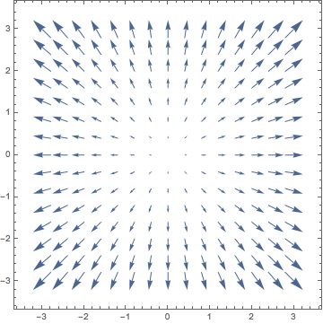
For example, if \(\boldsymbol{V}(x, y, z)) = (V_1(x, y, z), V_2(x, y, z), V_3(x, y, z))\) is a (three-dimensional) vector field, then \(\mathrm{div}(\boldsymbol{V})\) is the (scalar-valued) function \[\mathrm{div}(\boldsymbol{V}) = \boldsymbol{\nabla} \cdot\boldsymbol{V} = \pdv{V_{1}}{x} + \pdv{V_{2}}{y} + \pdv{V_{3}}{z} \,.\] The divergence tells us whether the flow (of air, fluid, etc.) represented by the vector field is (locally) expanding or contracting; that is, it is a measure of whether the vector field is (locally near a point) pushing away from a source (positive divergence) or towards a sink (negative divergence). This local expansion or contraction can be seen in whether the vectors in the vector field are converging or diverging locally near a given point as an expanding ball centred at the origin passes through that point.

💪 Try it out

If \(\boldsymbol{V}(x,y)= x \boldsymbol{i}+ y \boldsymbol{j}\), then \(\pdv{V_1}{x} = \pdv{x}{x} = 1\) and \(\pdv{V_2}{y} = \pdv{y}{y} = 1\), so \(\boldsymbol{\nabla} \cdot \boldsymbol{V} = 2\). Indeed, as we saw in the picture in the previous section, arrows in the vector field are diverging as we move away from the origin.

On the other hand, if \(\boldsymbol{V}(x,y) = -y \boldsymbol{i}+ x \boldsymbol{j}\), then we find \(\boldsymbol{\nabla} \cdot \boldsymbol{V} = 0\), so there is no divergence; that is, the vector field neither expands nor contracts (anywhere) as we move away from the origin. We sometimes call such a vector field divergenceless or divergence-free.

Note that the Laplacian of a scalar-valued function \(f(x_1, x_2, \dots, x_n)\) can also be understood as the divergence of its gradient, since \[\nabla^{2} f = \boldsymbol{\nabla}\cdot(\boldsymbol{\nabla} f) = \mathrm{div}(\boldsymbol{\nabla} f).\]

💪 Try it out

Compute \(\boldsymbol{\nabla} \cdot\boldsymbol{V}\) for \(\boldsymbol{V}=(x^{2}y,\,xyz,-x^{2}y^{2})\).

Answer:

From the definition, we find that \[\begin{aligned} \mathrm{div}(\boldsymbol{V}) = \boldsymbol{\nabla} \cdot\boldsymbol{V} &=\partial_{x}(x^{2}y)+\partial_{y}(xyz)+\partial_{z}(-x^{2}y^{2})\\ &=2xy+xz. \end{aligned}\] Note that the divergence is, indeed, a scalar-valued function whose value depends on the point \((x,y,z) \in \mathbb{R}^3\) in question.

5.3 Curl (of a 3-Dimensional field)

5.3.0.1 Interlude: determinants

Before getting into the curl, let’s recall how to compute the determinant of a matrix. The determinant of a \(2 \times 2\) matrix \(M\) is \[\det(M) = \left|\begin{array}{cc} M_{11} & M_{12}\\ M_{21} & M_{22} \end{array}\right| = M_{11}M_{22} - M_{12}M_{21} \,.\] To compute the determinant of a \(3 \times 3\) matrix, we go along the first row with alternating sign and then compute the determinants of the \(2 \times 2\) submatrices remaining when you ignore the first row and the columns corresponding to the entries on the first row: \[\begin{aligned} \left|\begin{array}{ccc} M_{11} & M_{12} & M_{13}\\ M_{21} & M_{22} & M_{23}\\ M_{31} & M_{32} & M_{33} \end{array}\right| & =M_{11} \left|\begin{array}{cc} M_{22} & M_{23}\\ M_{31} & M_{32} \end{array}\right| - M_{12}\left|\begin{array}{cc}M_{21} & M_{23}\\ M_{31} & M_{33} \end{array}\right| + M_{13} \left|\begin{array}{cc}M_{21} & M_{22}\\ M_{31} & M_{32} \end{array}\right| \\ &= M_{11}(M_{22}M_{33} - M_{23}M_{32}) - M_{12}(M_{21}M_{33}-M_{23}M_{31}) \\[1mm] &\hspace{35mm} + M_{13}(M_{21}M_{32}-M_{22}M_{31}). \end{aligned}\]

5.3.0.2 The curl

🔑 Key idea

The curl of a 3-dimensional vector field \(\boldsymbol{V}(x,y,z) = (V_1(x,y,z), V_2(x,y,z), V_3(x,y,z))\) is the 3-dimensional vector field defined by \[\begin{aligned} \mathrm{curl}(\boldsymbol{V}) & =\boldsymbol{\nabla}\times\boldsymbol{V} \qquad \text{(cross product)}\\ &=\left|\begin{array}{ccc} \boldsymbol{i} & \boldsymbol{j} & \boldsymbol{k}\\ \frac{\partial}{\partial x} & \frac{\partial}{\partial y} & \frac{\partial}{\partial z}\\ V_{1} & V_{2} & V_{3} \end{array}\right| \\[1mm] &=(\partial_{y}V_{3}-\partial_{z}V_{2})\boldsymbol{i}-(\partial_{x}V_{3}-\partial_{z}V_{1})\boldsymbol{j}+(\partial_{x}V_{2}-\partial_{y}V_{1})\boldsymbol{k}. \end{aligned}\] The curl is a measure of the rotation of the flow lines about an axis; i.e. how curly the field is!

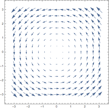
From the curl, we can read off the axis and direction of rotation of the vector field (at a given point) using the right-hand rule: point the thumb on your right hand in the direction of \(\mathrm{curl}(\boldsymbol{V})\) and curl your fingers closed. Then the axis of rotation points in the direction of your thumb and the rotation is in the same direction as the curl of your fingers.

💪 Try it out

We can imagine the vector field \(\boldsymbol{V}= x \boldsymbol{i}+ y \boldsymbol{j}\) to be in three dimensions by taking the component in the \(z\)-direction to be zero, i.e. \(\boldsymbol{V}= x \boldsymbol{i} + y\boldsymbol{j} + 0\boldsymbol{k}\). Then we have \[\boldsymbol{\nabla}\times\boldsymbol{V} = 0 \boldsymbol{i} + 0\boldsymbol{j} + \left(\partial_{x}y-\partial_{y}x\right)\boldsymbol{k}= = 0 \boldsymbol{i}+ 0 \boldsymbol{j} + 0 \boldsymbol{k}.\] This field has no rotation (and is said to be irrotational).

On the other hand, when \(\boldsymbol{V}= -y \boldsymbol{i}+ x \boldsymbol{j}\), we have \[\nabla\times\boldsymbol{V} = 0\boldsymbol{i}+0\boldsymbol{j}+\left(\partial_{x}x-\partial_{y}(-y)\right)\boldsymbol{k}=2\boldsymbol{k},\] i.e. a vector of length 2 pointing in the \(z\) direction. Then, by the right-hand rule, the vector field is rotating around the \(z\)-axis in an anti-clockwise direction (which we already knew from the picture!).

Unlike divergence, curl only works in three dimensions, because the cross product is defined only in three dimensions.

Now here are a few facts:

1. For any function \(f(x,y,z)\), we have \(\boldsymbol{\nabla}\times(\boldsymbol{\nabla} f)= \boldsymbol{0}\): i.e. the curl of a gradient is zero.

2. For any vector field \(\boldsymbol{V}(x,y,z)\), we have: \(\boldsymbol{\nabla}\cdot(\boldsymbol{\nabla}\times\boldsymbol{V})=0\), i.e. the divergence of a curl is zero.

These are not at all hard to prove by simply working everything out in components, and you are encouraged to do this. Here’s an example illustrating the second of these properties.

💪 Try it out

Compute \(\boldsymbol{\nabla}\times\boldsymbol{V}\) for \(\boldsymbol{V}(x,y,z)=(x^{2}y,\,xyz,-x^{2}y^{2})\) and verify that its divergence is zero.

Answer:

By definition, we have that \[\begin{aligned} \boldsymbol{\nabla}\times\boldsymbol{V} & =\left|\begin{array}{ccc} \boldsymbol{i} & \boldsymbol{j} & \boldsymbol{k}\\ \frac{\partial}{\partial x} & \frac{\partial}{\partial y} & \frac{\partial}{\partial z}\\ x^{2}y & xyz & -x^{2}y^{2} \end{array}\right|\\ &= (-2x^{2}y-xy) \boldsymbol{i}-(-2xy^{2}-0) \boldsymbol{j} + (yz-x^{2}) \boldsymbol{k}\\ &= (-xy(2x+1)\,,\,\,2xy^{2}\,,\,yz-x^{2}). \end{aligned}\] Note that the curl is a vector field. Now, the divergence of this vector field is \[\begin{aligned} \boldsymbol{\nabla}\cdot(\boldsymbol{\nabla}\times\boldsymbol{V}) & =-4xy-y+4xy+y\\ &= 0, \end{aligned}\] the constant-zero function, as expected.

5.4 Properties of div, grad and curl

We already saw a couple of these properties, but now that we have defined the divergence and curl, it is worth collecting all the properties together. These identities can be proved with simple product and chain rule applications.

1. \(\boldsymbol{\nabla}(f+g)=\boldsymbol{\nabla} f+\boldsymbol{\nabla} g\) (Distributivity of gradient)

2. \(\boldsymbol{\nabla}\cdot(\boldsymbol{V}+\boldsymbol{W})=\boldsymbol{\nabla}\cdot\boldsymbol{V}+\boldsymbol{\nabla}\cdot\boldsymbol{W}\) (Distributivity of divergence)

3. \(\boldsymbol{\nabla}\times(\boldsymbol{V}+\boldsymbol{W})=\boldsymbol{\nabla}\times\boldsymbol{V}+\boldsymbol{\nabla}\times\boldsymbol{W}\) (Distributivity of curl)

4. \(\boldsymbol{\nabla}(fg)=f\,\boldsymbol{\nabla} g+g\,\boldsymbol{\nabla} f\) Product rule for scalar functions)

5. \(\boldsymbol{\nabla}\cdot(f\boldsymbol{V})=f\,\boldsymbol{\nabla}\cdot\boldsymbol{V}+\left(\boldsymbol{\nabla} f\right)\cdot\boldsymbol{V}\) (Product rule for divergence of scalar times vector function)

6. \(\boldsymbol{\nabla}\times(f\boldsymbol{V})=f\,\boldsymbol{\nabla}\times\boldsymbol{V}+\left(\boldsymbol{\nabla} f\right)\times\boldsymbol{V}\) (Product rule for curl of scalar times vector function: note the ordering)

7. \(\boldsymbol{\nabla}\cdot(\boldsymbol{V}\times\boldsymbol{W})=\left(\boldsymbol{\nabla}\times\boldsymbol{V}\right)\cdot\boldsymbol{W}-\left(\boldsymbol{\nabla}\times\boldsymbol{W}\right)\cdot\boldsymbol{V}\) (Product rule for divergence of cross-products)

In addition there are simple identities for multiple applications of \(\boldsymbol{\nabla}\). Here are a few of the most commonly used, where the Laplacian \(\nabla^2 \boldsymbol{V}\) of a three-dimensional vector field \(\boldsymbol{V} = (V_1, V_2, V_3)\) is defined to be the vector field \((\nabla^2 V_1, \nabla^2 V_2, \nabla^2 V_3)\) given by taking the Laplacians of the individual coordinate functions.

1. \(\boldsymbol{\nabla}\cdot(\boldsymbol{\nabla} f)=\nabla^{2}f\). (The divergence of a gradient is the Laplacian.)

2. \(\boldsymbol{\nabla}\times(\boldsymbol{\nabla} f)= \boldsymbol{0}\). (Follows trivially from the definition of curl. The gradient of any field is irrotational.)

3. \(\boldsymbol{\nabla}\cdot(\boldsymbol{\nabla}\times\boldsymbol{V})=0\). (Again follows immediately from the definition of curl. The curl of any field is divergenceless.)

4. \(\boldsymbol{\nabla}\times(\boldsymbol{\nabla}\times\boldsymbol{V})=\boldsymbol{\nabla}(\boldsymbol{\nabla}\cdot\boldsymbol{V})-\nabla^{2}\boldsymbol{V}\) (This one is actually kind of important, as we will see in a second).

5. \(\boldsymbol{\nabla}\cdot(f\boldsymbol{\nabla} g)=f\nabla^{2}g+\boldsymbol{\nabla} f\cdot\boldsymbol{\nabla} g\)

6. \(\nabla^{2}(fg)=f\nabla^{2}g+2\boldsymbol{\nabla} f\cdot\boldsymbol{\nabla} g+g\nabla^{2}f\).

5.5 The Maxwell equations

These equations are the most famous physical example of where the concepts of divergence and curl are used, although they appear in many other areas, e.g. fluid mechanics.

It is a fact that there exist time-dependent vector fields in three-dimensional space called the electric field and magnetic field. At each (fixed) time \(t\), these vector fields are three-dimensional vector fields in the sense defined in Section 5.1 and, as \(t\) varies, the vector fields we see in space will evolve (think of the animated wind maps on the weather forecast). You have experienced such electric and magnetic fields already in your life: you know about magnets and static electricity and lightning and light and – honestly the list goes on. It turns out that essentially every single observable phenomenon¹ in everyday life is due to electromagnetism in some manner.

Famously, the electric field \(\boldsymbol{E}\) and magnetic field \(\boldsymbol{B}\) satisfy the Maxwell equations, which, in a vacuum (meaning there are no charges and no currents), take the following form:

\[\begin{aligned} \boldsymbol{\nabla}\cdot\boldsymbol{E} & =0\nonumber \\ \boldsymbol{\nabla}\cdot\boldsymbol{B} & =0\nonumber \\ \boldsymbol{\nabla}\times\boldsymbol{E} & =-\frac{\partial\boldsymbol{B}}{\partial t}\nonumber \\ \boldsymbol{\nabla}\times\boldsymbol{B} & =\frac{1}{c^{2}}\frac{\partial\boldsymbol{E}}{\partial t}\,\,.\label{eq:maxwell} \end{aligned}\] In these formulas, the constant \(c\) is the speed of light, which in conventional units has the value \(3 \times 10^{8} \mathrm{m} \mathrm{s}^{-1}\).

Why should this be the speed of light? It is because lurking in these equations, we can deduce that (the components of) the electric field \(\boldsymbol{E}\) and the magnetic field \(\boldsymbol{B}\) obey the (vector) wave equation, with speed \(c\). That is, for the electric field \(\boldsymbol{E}\) we have, on the one hand, \[\boldsymbol{\nabla}\times(\boldsymbol{\nabla}\times\boldsymbol{E}) = \boldsymbol{\nabla}(\boldsymbol{\nabla}\cdot\boldsymbol{E}) - \nabla^{2}\boldsymbol{E} = - \nabla^{2}\boldsymbol{E}\] and, on the other, \[\boldsymbol{\nabla}\times(\boldsymbol{\nabla}\times\boldsymbol{E}) = - \boldsymbol{\nabla}\times\frac{\partial\boldsymbol{B}}{\partial t} = - \frac{\partial}{\partial t}\left(\frac{1}{c^{2}}\frac{\partial\boldsymbol{E}}{\partial t}\right) = - \frac{1}{c^{2}}\frac{\partial^{2}\boldsymbol{E}}{\partial t^{2}},\] which together yield \[\frac{\partial^{2}\boldsymbol{E}}{\partial t^{2}} = c^2 \, \nabla^{2}\boldsymbol{E}\,.\] A similar computation will show that the magnetic field \(\boldsymbol{B}\) must also satisfy the (same) wave equation. Therefore, it follows that inserting a consistent d’Alembert solution to the (scalar) wave equation into each component of \(\boldsymbol{E}\) and \(\boldsymbol{B}\) should lead toward solutions of the Maxwell equations.

We can check to see what this means, although we need to be a little careful if/when trying to apply rules for scalar-valued functions from the previous section to vector fields. Let \(f(s)\) be an arbitrary (twice-differentiable) function of one variable and let \(\boldsymbol{\hat v}\) be a unit vector (i.e. \(\boldsymbol{\hat v} \cdot \boldsymbol{\hat v} = 1\)) pointing in the desired direction of travel of our wave. Furthermore, let \(\boldsymbol{E_0}\) and \(\boldsymbol{B_0}\) be fixed (i.e. constant) three-dimensional vectors. Now consider the vector fields \(\boldsymbol{E}\) and \(\boldsymbol{B}\) defined at \(\mathbf{x} \in \mathbb{R}^3\) by \[\boldsymbol{E}(\mathbf{x}, t) = f(\hat{\boldsymbol{v}}\cdot\mathbf{x}-ct) \, \boldsymbol{E_0} \quad \text{ and } \quad \boldsymbol{B}(\mathbf{x}, t) = f(\hat{\boldsymbol{v}}\cdot\mathbf{x}-ct) \, \boldsymbol{B_0} \,.\]

Using the definition of the Laplacian for vector fields in the previous section, it is not difficult to compute that \[\nabla^{2}\boldsymbol{E} = f''(\boldsymbol{\hat v}\cdot\mathbf{x}-ct) \, \boldsymbol{E}_{0}\] and, by the chain rule, that \[\frac{\partial^{2}\boldsymbol{E}}{\partial t^{2}} = c^{2} f''(\boldsymbol{\hat v}\cdot\mathbf{x}-ct) \, \boldsymbol{E}_{0} \,,\] and analogously for \(\boldsymbol{B}\). Thus, the wave equation is certainly satisfied by both \(\boldsymbol{E}\) and \(\boldsymbol{B}\).

However, the Maxwell equations actually contain more information since \[0 = \boldsymbol{\nabla}\cdot\boldsymbol{E} = f''(\boldsymbol{\hat v}\cdot\mathbf{x}-ct) \, \boldsymbol{\hat{v}}\cdot\boldsymbol{E}_{0}\,.\] This tells us that \(\boldsymbol{\hat{v}}\cdot\boldsymbol{E}_{0}=0\), so that the electric field \(\boldsymbol{E}\) (which is parallel to \(\boldsymbol{E_0}\)) is orthogonal to the direction \(\boldsymbol{\hat v}\) in which the wave is travelling.

The fourth Maxwell equation now tells us \[f'(\boldsymbol{\hat v}\cdot\mathbf{x}-ct) \, \boldsymbol{\hat{v}}\times\boldsymbol{B_{0}} = \boldsymbol{\nabla}\times\boldsymbol{B} = \frac{1}{c^{2}}\frac{\partial\boldsymbol{E}}{\partial t} = - \frac{1}{c} f'(\hat{\boldsymbol{k}}\cdot\mathbf{x}-ct) \, \boldsymbol{E}_{0}\] which implies that \[c \, \boldsymbol{B_{0}} \times \boldsymbol{\hat{v}} = \boldsymbol{E}_{0}\,.\] Therefore, we may conclude that the electric field \(\boldsymbol{E}\) (which is parallel to \(\boldsymbol{E_0}\)), the magnetic field \(\boldsymbol{B}\) (which is parallel to \(\boldsymbol{B_0}\)) and the direction \(\boldsymbol{\hat{v}}\) are all mutually orthogonal. In other words, if there is a wave propagating in space in a direction \(\boldsymbol{\hat v}\), then these electric and magnetic fields are both concentrated in the plane perpendicular to that direction.

---

1. Except those involving gravity; gravity and electromagnetism are the only long-range forces in the universe.