1 Axioms of probability

🥅 Goals

Understand elementary set theory and how to use it to formulate probabilistic scenarios and to describe the calculus of events.
Be familiar with the axioms of probability and their consequences, and how these properties may be deduced from the axioms.

In this chapter, we lay the foundations of probability calculus, and establish the main techniques for practical calculations with probabilities. The mathematical theory of probability is based on axioms, like Euclidean geometry. In classical geometry, the fundamental objects posited by the axioms are points and lines; in probability, they are events and their probabilities. The language and apparatus of set theory is used to express these concepts and to work with them.

There is a lot of ambiguity inherent in probability, because we are often using mathematical approaches to describe real-world scenarios. In some cases, there are several different ways to represent the real-world scenario as a probabilistic model, and the choices we make could affect our conclusions. In others, an unambiguous mathematical setup could have different real-world interpretations, depending on how we view it. Either way, once we have a probabilistic model, the axioms help us to ensure that the maths remains the same.

The axioms and properties of probability we develop in this chapter lay the foundations for all the rest of the theory we will build later in the course.

1.1 Sets

One of the key tools we need in this chapter is a good understanding of set theory. You’ll see all of this much more formally in Analysis, but in this section we give a quick rundown of the essentials we need for Probability.

In essence, a set is an unordered collection of distinguishable objects; these objects can be numbers, functions, other sets, and so on—any mathematical object can belong to a set.

The formal notation for a set is an opening curly bracket, followed by a list of elements that belong to the set, followed by a closing curly bracket. For instance, the set containing the elements $2$, $4$, and $5$ is denoted by \[ \{2,4,5\}. \] Because the ordering of the elements is irrelevant, $\{2,4,5\}$ and $\{4,5,2\}$ denote the same set.

Definition: empty set

The set with no outcomes is called the empty set, and is denoted by $\emptyset$: \[ \emptyset:=\{\}. \]

A set is often denoted by a capital letter such as $A$, $B$, $C$, and so on.

Definition: subset

For two sets $A$ and $B$, we say that $A$ is a subset of $B$, and we write $A\subseteq B$ (or $B\supseteq A$), whenever every element that belongs to $A$ also belongs to $B$, that is, for all $x \in A$ we have $x \in B$.

For instance, $\{2,4,5\}\subseteq\{1,2,3,4,5\}$. Note that for every set $A$, we have $A \subseteq A$ and $\emptyset\subseteq A$. We can also use strict subsets, when the subset is not equal to the larger set: $\{2,4,5\} \subset \{1,2,3,4,5\}$.

Definition: power set

The set consisting of all subsets of a set $A$ is called the power set of $A$, and is denoted as $2^A$: \[ 2^A:=\{B\colon B\subseteq A\}. \]

For example, the power set of the set $A=\{1,2,3\}$ is \[ 2^A=\{\emptyset,\{1\},\{2\},\{3\},\{1,2\},\{1,3\},\{2,3\},\{1,2,3\}\}. \]

The notation $2^A$ alludes to the size of the power set. When $A$ is a finite set, its power set contains $2^{|A|}$ subsets. This can be proved by constructing a bijection from $2^A$ to ordered $|A|$-tuples of $0$s and $1$s, where a $1$ indicates that the corresponding element of $A$ is in the subset.

📖 Textbook references

If you want more help with this section, check out:

Appendix A.1 in (Blitzstein and Hwang 2019);
Appendix B in (Anderson, Seppäläinen, and Valkó 2018);
or the Appendix to Chapter 0 in (Stirzaker 2003).

1.2 Sample space and events

Definition: scenarios, outcomes and sample space

Whenever we do some probability, it is based on a scenario in which there are various outcomes. We assume that we know the (set of all) possible outcomes, but we are unsure about which outcome will occur.

A sample space is a set of outcomes for this scenario with the property that one (and only one) of these outcomes must occur.

In this course, we will usually denote the sample space by $\Omega$, and a generic outcome by $\omega \in \Omega$.

For instance, suppose we roll a standard six-sided die.

The most obvious sample space is $\Omega = \{1,2,3,4,5,6\}$, but if one was interested only in whether the die was odd or even, or a six or not, one could use $\Omega = \{\text{odd},\text{even}\}$, or $\Omega = \{\text{not a }6, 6\}$.

Often, like in the above example, we may enumerate the elements of the sample space $\Omega$ in a finite or infinite list $\Omega = \{ \omega_1, \omega_2, \ldots \}$, in which case we say the set $\Omega$ is countable or discrete.

A set is said to be countable when its elements can be enumerated in a (possibly infinite) sequence. Every finite set is countable, and so is the set of natural numbers $\mathbb{N} := \{1,2,3,\ldots \}$. The set of integers $\mathbb{Z}$ is countable as well. The set of real numbers $\mathbb{R}$ is not countable, and neither is any interval $[a,b]$ when $a<b$.

Definition: countable

A set $A$ is countable if either:

$A$ is finite, or
there is a bijection (one-to-one and onto mapping) between $A$ and the set of natural numbers $\mathbb{N}$.

One can prove that the set of rational numbers $\mathbb{Q}$ is countable.

When we perform an experiment we are interested in the occurence, or otherwise, of events. An event is just a collection of possible outcomes, i.e., a subset of $\Omega$.

🔑 Key idea: Definition: events

Associated to our sample space $\Omega$ is a collection $\mathcal{F}$ of events: \[ A \subseteq \Omega \text{ for every } A \in \mathcal{F}. \] We say that an event $A$ occurs when the outcome that occurs at the end of the scenario is in the set $A$.

If $\Omega$ is discrete, we can always take $\mathcal{F} = 2^\Omega$, so that every subset of $\Omega$ is an event. If $\Omega$ is not discrete, we need to be a little more careful: see Section 1.4 below.

The empty set $\emptyset$ represents the impossible event, i.e., it will never occur. The sample space $\Omega$ represents the certain event, i.e., it will always occur. Most interesting events are somewhere in between.

The representation of an event as a set obviously depends on the choice of sample space $\Omega$ for the specific scenario under study, as shown by the following two examples.

Examples

For rolling a standard cubic die (with $\Omega=\{1,2,3,4,5,6\}$), the event “throw an odd number” is the subset $A = \{1,3,5\}$ consisting of three outcomes. If we roll the die and it comes up a 3, then event $A$ has occurred.
For the same scenario, but with $\Omega=\{\text{odd},\text{even}\}$, the event ‘throw an odd number’ is the subset $A = \{\text{odd}\}$ consisting of just one outcome.

💪 Try it out

Suppose we roll three standard six-sided dice and record the outcome of the experiment by an ordered triple $(i,j,k)$ where $i,j,k \in \{1,2,\ldots,6\}$. What is $\Omega$? How big could $\mathcal{F}$ be?

Answer:

In this case $\Omega = \{1,2,\ldots,6\}^3$ has $6^3 = 216$ individual outcomes.

The number of events ($2^{216}$) is enormous! One is the event that the scores on the three dice are the same: $A = \{ (1,1,1), (2,2,2), \ldots, (6,6,6) \}$.

📖 Textbook references

If you want more help with this section, check out:

Section 1.2 in (Blitzstein and Hwang 2019);
Section 1.1 in (Anderson, Seppäläinen, and Valkó 2018);
Sections 1.1 and 1.2 in (Stirzaker 2003);
or Section 1.4 in (DeGroot and Schervish 2013).

1.3 Event calculus

Once we’ve defined our sample space and the set of all possible events, we need to be able to refer to combinations of events. To do so, we use standard notation from set theory.

Definition: complements

For an event $A \in \mathcal{F}$, we define its complement, denoted $A^\mathrm{c}$ (or sometimes $\bar A$) and read “not $A$”, to be \[A^\mathrm{c} := \Omega \backslash A = \{ \omega \in \Omega : \omega \notin A\}.\]

Notice that:

the complement of $A^\mathrm{c}$ is $A$: $(A^\mathrm{c})^\mathrm{c}=A$;
there are no outcomes in both $A$ and $A^\mathrm{c}$: $A \cap A^\mathrm{c} = \emptyset$;
and every outcome is in one or the other: $A \cup A^\mathrm{c} = \Omega$.

🔑 Key idea: event calculus

Given any two events $A$ and $B$ that are associated with the same sample space (i.e. $A\subseteq\Omega$ and $B\subseteq\Omega$ for the same $\Omega$), here are some of the other events we can define, along with how we would read them out:

Notation	We say (as sets)	We say (as events)	Meaning (as events)
$A \cup B$	$A$ union $B$	$A$ or $B$	$A$ occurs or $B$ occurs or both $A$ and $B$ occur
$A \cap B$	$A$ intersect $B$	$A$ and $B$	$A$ occurs and $B$ occurs
$A^\mathrm{c} := \Omega \backslash A$	$A$ complement	not $A$	$A$ does not occur
$A\backslash B$	$A$ minus $B$	$A$ but not $B$	$A$ occurs but $B$ does not
$A\subseteq B$	$A$ is a subset of $B$	$A$ implies $B$	if $A$ occurs, then $B$ must occur

(In the final row, “$A \subseteq B$” is not an event but rather a statement about how two events relate to each other. I still wanted to include it because I think it’s helpful)

💪 Try it out

Prove that $A \backslash B = A \cap B^\mathrm{c}$.

Answer:

We can do this by working with the events as sets. We have \[ A \backslash B = \{ \omega \in \Omega : \omega \in A, \, \omega \notin B \} = \{ \omega \in \Omega : \omega \in A \} \cap \{ \omega \in \Omega : \omega \notin B \} = A \cap B^\mathrm{c} . \]

🔑 Key idea: Definition: disjoint

We say that events $A$ and $B$ are disjoint, mutually exclusive, or incompatible if $A \cap B = \emptyset$, i.e., it is impossible for $A$ and $B$ both to occur.

💪 Try it out

Consider the sample space $\Omega:=\{1,2,3,4,5,6\}$, and the events \[\begin{align*} A&:=\{2,4,6\}, \\ B&:=\{1,3,5\}, \\ C&:=\{1,2,3\}. \end{align*}\] In other words, $A$ is the event “throw an even number”, $B$ is the event “throw an odd number”, and $C$ is the event “throw at most three”. Use some of the ideas from the table above to combine events $A$, $B$, and $C$ in different ways. Are any of your new events disjoint?

Answer:

Some combinations: \[\begin{align*} A\cup B&=\Omega && \text{(even or odd)} \\ A\cap B&=\emptyset && \text{(even and odd)} \\ A^\mathrm{c}&=B && \text{(not even)} \\ C\backslash A&=\{1,3\} && \text{(at most 3 but not even)} \\ A\cup C&=\{1,2,3,4,6\} && \text{(even or at most 3)} \\ A\cap C&=\{2\} && \text{(even and at most 3)}. \end{align*}\] The events $A$ and $B$ are disjoint as $A\cap B=\emptyset$. We have also created two disjoint events: $C\backslash A$ and $A \cap C$. Think about why these two events would always be disjoint, however we define $A$ and $C$.

💪 Try it out

Toss a coin twice and denote the sample space by $\Omega = \{ \text{HH}, \text{HT}, \text{TH}, \text{TT} \}$. Consider the events \[\begin{align*} A & := \{ \text{HH}, \text{HT} \} && \text{(first toss H)} \\ B & := \{ \text{HT}, \text{TT} \} && \text{(second toss T)} \\ C & := \{ \text{HH} \} && \text{(both H)} .\end{align*}\] How do these events relate to each other?

Answer:

Some things you might notice:

$C \subseteq A$, i.e., if $C$ occurs then $A$ must occur;
$A \cup B = \{ \text{HH}, \text{HT}, \text{TT} \}$ is the event that either the first toss is H, the second toss is T, or both;
$A \cap B = \{ \text{HT} \}$;
$A^\mathrm{c} = \{ \text{TH}, \text{TT} \}$;
$B \cap C = \emptyset$.

💪 Try it out

Draw a card from a standard deck of 52 playing cards. Take $\Omega$ to consist of each of the 52 possible draws: $\Omega = \{ \text{A}\clubsuit, \text{A}\diamondsuit, \ldots , \text{K}\heartsuit, \text{K}\spadesuit\}$. Events in $\mathcal{F} = 2^\Omega$ include \[\begin{align*} E & = \{ \text{eight} \} = \{ 8\spadesuit,8\heartsuit,8\diamondsuit,8\clubsuit \} ,\\ S & = \{ \text{spade} \} = \{A\spadesuit,2\spadesuit, \ldots, K\spadesuit\} , \end{align*}\] and we can combine them to form other events, such as \[\begin{align*} E \cap S & = \{ 8\spadesuit \}, \\ E\backslash S &= \{8\heartsuit, 8\diamondsuit, 8\clubsuit \}, \\ S\backslash E &= \{A\spadesuit,2\spadesuit,\dots,7\spadesuit,9\spadesuit,\dots,K\spadesuit\}. \end{align*}\]

As with sums ($\sum$) and products ($\Pi$) of multiple numbers, we also have shorthands for unions and intersections of multiple sets: \[ \bigcup_{i=1}^n A_i:= A_1\cup A_2\cup\dots\cup A_n \] is the event that at least one of $A_1, A_2, \dots A_n$ occurs (or the set of all $\omega \in \Omega$ which are contained in at least one of the $A_i$s), and \[ \bigcap_{i=1}^n A_i:= A_1\cap A_2\cap\dots\cap A_n \] is the event that all of $A_1, A_2, \dots A_n$ occur (or the set of all $\omega \in \Omega$ which are in every $A_i$).

Occasionally, we will also need to take infinite unions and intersections over sequences of sets: \[\begin{align*} \bigcup_{i=1}^\infty A_i&:= A_1\cup A_2\cup A_3\cup\dots \\ \bigcap_{i=1}^\infty A_i&:= A_1\cap A_2\cap A_3\cap\dots. \end{align*}\]

We will also sometimes need De Morgan’s Laws: for a (possibly infinite) collection of events $A_i$,

The complement of the union is the intersection of the complements: $\left( \bigcup_{i} A_i \right)^\mathrm{c} = \bigcap_i A_i^\mathrm{c}$, and
The complement of the intersection is the union of the complements: $\left( \bigcap_{i} A_i \right)^\mathrm{c} = \bigcup_i A_i^\mathrm{c}$.

These could be more intuitive than they appear: the negation of “some of these things happened” is “none of these things happened”, and the negation of “all of these things happened” is “some of these things did not happen”.

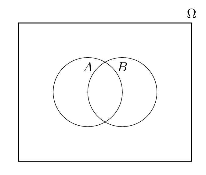
It is often useful to visualize the sample space in a Venn diagram. Then events such as $A$ are subsets of the sample space. It is a helpful analogy to imagine the probability of an event as the area in the Venn diagram.

Advanced content

This analogy is more apt than it first appears, since the mathematical foundations of rigorous probability theory are built on measure theory, which is the same theory that gives rigorous foundation to the concepts of length, area, and volume.

📖 Textbook references

If you want more help with this section, check out:

Section 1.2 in (Blitzstein and Hwang 2019);
Section 1.2 in (Stirzaker 2003);
or Section 1.4 in (DeGroot and Schervish 2013).

1.4 Sigma-algebras

In the last section we described some of the ways in which events can be combined. Now we can set out the rules for our collection of events, $\mathcal{F}$, to ensure that it’s possible to use these different combinations.

We said that in the case where $\Omega$ is discrete, one can take $\mathcal{F} = 2^\Omega$.

In general, if $\Omega$ is uncountable, it is too much to demand that probabilities should be defined on all subsets of $\Omega$. The reason why this is a problem goes beyond the scope of this course (see the Bibliographical notes at the end of this chapter for references), but the essence is that for uncountable sample spaces, such as $\Omega=[0,1]$, there exist subsets of $\Omega$ that cannot be assigned a probability in a way that is consistent. The construction of such non-measurable sets is also the basis of the famous Banach–Tarski paradox.

Uncountable $\Omega$ are unavoidable: we will see an infinite coin-tossing space at the end of section Section 1.6, and other examples occur whenever we have an experiment whose outcome is modelled by a continuous distribution such as the normal distribution (more on this later).

The upshot of all this is that we can, in general, only demand that probabilities are defined for all events in some collection $\mathcal{F}$ of subsets of $\Omega$ (i.e., for some $\mathcal{F} \subseteq 2^\Omega$). What properties should the collection $\mathcal{F}$ of events possess? Consideration of the set operations in the previous section suggests the following definition.

Definition: σ-algebra

A collection $\mathcal{F}$ of subsets of $\Omega$ is called a $\sigma$-algebra over $\Omega$ if it satisfies the following properties.

(S1) $\Omega \in \mathcal{F}$;

(S2) $A \in \mathcal{F}$ implies that $A^\mathrm{c} \in \mathcal{F}$;

(S3) if $A_1, A_2, \ldots \in \mathcal{F}$ then $\bigcup_{i=1}^\infty A_i \in \mathcal{F}$.

Property S2 says that $\mathcal{F}$ is closed under complementation, while S3 says that $\mathcal{F}$ is closed under countable unions.

We can combine S1 and S2 to see that we must have $\emptyset \in \mathcal{F}$. Also note that, we can get to a finite-union version of S3 by taking $A_{n+1} = A_{n+2} = \cdots = \emptyset$: so $\mathcal{F}$ is also closed under finite unions.

Examples

The power set $2^\Omega$ is a $\sigma$-algebra over $\Omega$, and in fact it is the biggest possible $\sigma$-algebra over $\Omega$. As described above, for uncountable $\Omega$ the set $2^\Omega$ may be too unwieldy, in which case we would consider a smaller $\sigma$-algebra.
The trivial $\sigma$-algebra $\{ \emptyset, \Omega \}$ is the smallest possible $\sigma$-algebra over $\Omega$. It’s very nicely behaved (just two elements!) but it carries no information about the outcome of the experiment.

💪 Try it out

Consider the sample space $\Omega = \{1,2,3,4,5,6\}$ for the experiment of rolling a fair die. The choice of $\sigma$-algebra determines the resolution at which we observe the experiment, and may depend on exactly what we are interested in:

$\mathcal{F}_0 = \{ \emptyset, \Omega \}$ (carries no information);
$\mathcal{F}_1 = \{ \emptyset, \{1,3,5\}, \{2,4,6\}, \Omega \}$ (if we only care whether the score is odd or even);
$\mathcal{F}_2 = 2^\Omega$ (if we are interested in the exact score).

Note the inclusions $\mathcal{F}_0 \subset \mathcal{F}_1 \subset \mathcal{F}_2$.

Let us check that $\mathcal{F}_1$ is indeed a $\sigma$-algebra.

S1 is immediate: we can see it from the definition of $\mathcal{F}_1$.

For S2, we need that every $A \in \mathcal{F}_1$ is accompanied by its complement $A^\mathrm{c}$; we see that this is the case.

Since $\mathcal{F}_1$ is a finite set it suffices to check S3 for finite unions. In other words, it is enough to check that if $A, B \in \mathcal{F}_1$, then $A \cup B \in \mathcal{F}_1$ too. Since there are only two sets, this is also quick: we see that it is the case.

📖 Textbook references

If you want more help with this section, check out:

Section 1.2 in (Stirzaker 2003).

1.5 The axioms of probability

🔑 Key idea: Definition: probability

A probability $\mathbb{P}{}$ on a sample space $\Omega$ with collection $\mathcal{F}$ of events is a function mapping every event $A \in \mathcal{F}$ to a real number $\mathbb{P}(A)$, obeying the following axioms:

(A1) $\mathbb{P}(A) \geq 0$ for every $A\in\mathcal{F}$;

(A2) $\mathbb{P}(\Omega) = 1$; and

(A3) if $A$ and $B$ are disjoint events (i.e. if $A, B \in \mathcal{F}$ have $A\cap B=\emptyset$) then \[ \mathbb{P}(A \cup B) = \mathbb{P}(A) + \mathbb{P}(B). \] We call the number $\mathbb{P}(A)$ the probability of $A$.

We will see shortly that a consequence of these axioms is that the probabilities $\mathbb{P}(A)$ must lie between $0$ and $1$: $0 \leq \mathbb{P}(A) \leq 1$.

We can upgrade (A3) to a slightly more technical version:

(A4) For any infinite sequence $A_1,A_2,\dots$ of pairwise disjoint events (so $A_i \cap A_j = \emptyset$ for all $i \neq j$), \[ \mathbb{P}\left( \bigcup_{i=1}^{\infty}A_i \right) = \sum_{i=1}^{\infty}\mathbb{P}(A_i). \]

🔑 Key idea: A small request

If you only take one thing away from this course, please let it be this:

Probabilities are numbers and events are sets.

We can add up numbers (but not sets) and we can take unions and intersections of sets (but not numbers).

For the axioms to make sense, we can’t just use any old event set $\mathcal{F}$. For one thing, we need $\Omega \in \mathcal{F}$; in fact all the events in (A1-4) need to be in $\mathcal{F}$. Our definition of a $\sigma$-algebra from the previous section gives us exactly the event set we need.

🔑 Key idea: Definition: probability space

If $\Omega$ is a set and $\mathcal{F}$ is a $\sigma$-algebra of subsets of $\Omega$, and if $\mathbb{P}$ satisfies (A1–4) for events in $\mathcal{F}$, then the triple $(\Omega, \mathcal{F}, \mathbb{P})$ is called a probability space.

💪 Try it out

Consider a finite sample space $\Omega = \{ \omega_1, \ldots, \omega_m\}$ of size $|\Omega|=m$. Then we can define a valid probability $\mathbb{P}$ by taking any numbers $p_1, \ldots, p_m$ with $p_i \geq 0$ for all $i$ and $\sum_{i=1}^m p_i = 1$ and declaring that for any event $A$, \[ \mathbb{P}(A) = \sum_{i : \omega_i \in A} p_i .\]

This satisfies the axioms (A1–4) (don’t just believe me - check them for yourself).

By considering the event $A = \{ \omega_i\}$, we see that $p_i = \mathbb{P}(\omega_i)$ is the probability of the elementary outcome $\omega_i$.

In the simplest setting, we might assume that all the outcomes are equally likely, that is, $p_i = 1/m$ for all $i$. Note that in this case probability reduces to counting, since \[ \mathbb{P}(A) = \sum_{i : \omega_i \in A} \frac{1}{m} = \frac{|A|}{|\Omega|} .\]

As a concrete example, for tossing a fair die we would have $\Omega = \{ 1,2,\ldots,6\}$, and $\mathbb{P}(A) = |A|/6$ so, for example, \[ \mathbb{P}(\text{score is odd})=\mathbb{P}(\{1,3,5\})= \frac{3}{6} = \frac{1}{2}. \] We examine this setting in detail in Chapter 2.

💪 Try it out

Consider a countably infinite sample space $\Omega = \{ \omega_1, \omega_2, \ldots \}$. Then we can define a valid probability $\mathbb{P}$ by taking any numbers $p_1, p_2, \ldots$ with $p_i \geq 0$ for all $i$ and $\sum_{i=1}^\infty p_i = 1$ and declaring that for any event $A$, \[ \mathbb{P}(A) = \sum_{i : \omega_i \in A} p_i .\]

This definition of a probability satisfies all of the axioms (A1-A4).

For this course, we will usually assume that the probability distribution is given (and satisfies the axioms), without worrying too much about how the important practical task of finding the probabilities was carried out.

📖 Textbook references

If you want more help with this section, check out:

Section 1.6 in (Blitzstein and Hwang 2019);
Section 1.1 in (Anderson, Seppäläinen, and Valkó 2018);
or Section 1.3 in (Stirzaker 2003).

1.6 Consequences of the axioms

A host of useful results can be derived from A1–4.

🔑 Key idea: Consequences of the axioms

(C1) For any two events $A$ and $B$, \[ \mathbb{P}(B \backslash A)=\mathbb{P}(B) - \mathbb{P}(A \cap B). \]

(C2) For any event $A$, $\mathbb{P}(A^\mathrm{c}) =1 - \mathbb{P}(A)$.

(C3) The probability of $\emptyset$ is $\mathbb{P}(\emptyset) = 0$.

(C4) For any event $A$, $\mathbb{P}(A) \leq 1$.

(C5) If $A \subseteq B$ then $\mathbb{P}(A) \leq \mathbb{P}(B)$ (“monotonicity”).

(C6) For any two events $A$ and $B$, \[ \mathbb{P}(A \cup B) = \mathbb{P}(A) + \mathbb{P}(B) - \mathbb{P}(A \cap B). \]

(C7) If $A_1, A_2, \dots, A_k$ are pairwise disjoint (so $A_i \cap A_j = \emptyset$ if $i \neq j$) then \[ \mathbb{P}\left(\bigcup_{i=1}^{k}A_i\right) = \sum_{i=1}^{k}\mathbb{P}(A_i). \] (This property is called “finite additivity” in textbooks.)

(C8) For any events $A_1, A_2, \ldots$, (these need not be pairwise disjoint), \[ \mathbb{P}( \bigcup_{i=1}^{\infty} A_i ) \leq \sum_{i=1}^{\infty}\mathbb{P}(A_i). \] (This one is sometimes referred to as “Boole’s inequality.”)

(C9) If $A_1 \subseteq A_2 \subseteq \cdots$ is an increasing sequence of events, then \[ \mathbb{P}\left( \bigcup_{n=1}^\infty A_n \right) = \lim_{n \to \infty} \mathbb{P}( A_n) . \] If $A_1 \supseteq A_2 \supseteq \cdots$ is a decreasing sequence of events, then \[ \mathbb{P}\left(\bigcap_{n=1}^\infty A_n \right) = \lim_{n \to \infty} \mathbb{P}(A_n) . \] (This property is a bit more sophisticated than the previous ones. It establishes the “continuity of probability along monotone limits:” we can take limits, as long as the events in question form a monotone sequence. It will be really important in Probability II.)

Just one more consequence to go! Before we get there, we need the following simple but extremely useful idea: partitions.

🔑 Key idea: Definition: partition

We say that the events $E_1, E_2, \ldots, E_k \in \mathcal{F}$ form a (finite) partition of the sample space $\Omega$ if:

they all have positive probability, i.e., $\mathbb{P}(E_i) >0$ for all $i$;
they are pairwise disjoint, i.e., $E_i\cap E_j=\emptyset$ whenever $i\neq j$; and
their union is the whole sample space: $\cup_{i=1}^k E_i=\Omega$.

The definition extends to countably infinite partitions. We say that $E_1, E_2, \ldots \in \mathcal{F}$ form an infinite partition of $\Omega$ if:

$\mathbb{P}(E_i) >0$ for all $i$;
$E_i\cap E_j=\emptyset$ whenever $i\neq j$; and
$\cup_{i=1}^\infty E_i=\Omega$.

For example, consider the sample space $\Omega=\{1,2,3,4,5,6\}$. Some partitions are: \[\begin{align*} \{1\}, \{2\}, \{3\}, \{4\}, \{5\}, \{6\} \\ \{1, 2\}, \{3, 4\}, \{5, 6\} \\ \{1, 2, 3\}, \{4, 5, 6\} \\ \{1\}, \{2, 3\}, \{4, 5, 6\} \\ \{1, 2, 3, 4, 5, 6\} \\ \end{align*}\] and so on.

🔑 Key idea

(C10) If $E_1$, $E_2$, , $E_k$ form a partition then \[ \sum_{i=1}^{k}\mathbb{P}(E_i)=1. \]

These consequences have an enormous effect on the way we work with probability. In particular, it turns out that we can solve most problems without ever having to explicitly write down the outcomes in our sample space, as in the next example. In fact, some people do probability without even defining a sample space.

💪 Try it out

Jimmy’s die has the numbers 2,2,2,2,5,5. Your die has numbers 1,1,4,4,4,4. You both throw and the highest number wins. Assuming all outcomes are equally likely, what is the probability that Jimmy wins?

Answer:

The event, $J$, that Jimmy wins happens if either Jimmy throws a 5 (call this event $F$), or if you throw a 1 (call this event $A$). Therefore $J = A \cup F$ and by C6, \[\mathbb{P}(J) = \mathbb{P}(A) + \mathbb{P}(F) - \mathbb{P}(A \cap F).\]
As $\mathbb{P}(F) = 1/3$, $\mathbb{P}(A) = 1/3$ and $\mathbb{P}(A\cap F) = 4/36 = 1/9$ (by counting equally likely outcomes) we have \[\mathbb{P}(J) = 1/3 + 1/3 - 1/9 = 5/9.\]

Finite sample spaces are a great way to build up our intuition for probability calculations. However, it is surprisingly easy to end up in a situation where things start to get complicated.

💪 Try it out

What is the probability that, in an indefinitely long sequence of tosses of a fair coin, we will eventually see heads?

Answer:

The sample space $\Omega$ is infinite and consists of all sequences $\omega = (\omega_1, \omega_2, \ldots)$ with $\omega_i \in \{ \text{H}, \text{T} \}$.

What is $\mathbb{P}$? Well, it certainly would be desirable that if we restrict to just a finite sequence of $n$ tosses, then each of the $2^n$ possible outcomes (sequences) should be equally likely. It is a special case of a general theorem that such a $\mathbb{P}$ exists and is unique.

Now, let $A = \{\text{H occurs}\}$. Then the only way $A$ can not occur is if there are no heads, i.e., $A^\mathrm{c} = \{ (\text{TTT$\cdots$} ) \}$. This is a single sequence, out of infinitely many, and it is intuitively clear that it should have probability $0$. To prove this, it is enough to observe that $A^\mathrm{c} \subseteq \{ \text{first } n \text{ tosses T}\}$, so by monotonicity (C5), \[ \mathbb{P}(A^\mathrm{c}) \leq \mathbb{P}( \{ \text{first } n \text{ tosses are T}\} ) \leq 2^{-n} .\] But this is true for any $n$, so we must have $\mathbb{P}(A^\mathrm{c}) =0$.

Another way to see this is as follows. Consider events defined for $n =1,2,\ldots$ by \[ A_n = \{\text{first H occurs on toss } n \} = \{ \omega : \omega_k = \text{T, for all } k < n, \, \omega_n = \text{H} \} .\] This means that $A_1$ consists of sequences H$\cdots$, $A_2$ consists of sequences TH$\cdots$, and so on.

Now the event we are interested in is $A = \cup_{n=1}^\infty A_n$. So, by (A4), \[ \mathbb{P}(A) = \sum_{n=1}^\infty \mathbb{P}(A_n) = \sum_{n=1}^\infty 2^{-n} = 1.\] Note that a similar argument works if the coin is biased with probability $p \in (0,1)$ of heads.

Advanced content

In fact, the sequence space $\Omega$ in the previous example is not even countable! To see this, a sequence $(d_1,d_2, \ldots)$ with each $d_i \in \{0,1\}$ is called a dyadic expansion of $x \in [0,1]$ if $x = \sum_{i=1}^\infty 2^{-i} d_i$. For example, $(1,0,0,\ldots)$ is a dyadic expansion of $1/2$, $(1,1,0,0,\ldots)$ is $3/4$, and so on. The map between $x$ and $(d_1,d_2,\ldots)$ is almost a bijection. It is not a bijection because of possible non-uniqueness of the dyadic expansion: e.g. $(0,1,1,1,\ldots)$ is another expansion of $1/2$. It turns out that this problem only occurs for rational $x$, and can be circumvented. Thus we have (essentially) a bijection between $[0,1]$ and the space of infinite sequences of $0$s and $1$s, which is another name for our coin tossing space $\Omega$. This shows that $\Omega$ is uncountable.

It is remarkable that the probability $\mathbb{P}$ on infinite sequences of coin tosses turns out to correspond (under the bijection by dyadic expansion) to nothing other than the uniform distribution on $[0,1]$, that is the measure defined by lengths of intervals. This is the famous Lebesgue measure.

📖 Textbook references

If you want more help with this section, check out:

Section 1.6 in (Blitzstein and Hwang 2019);
Section 1.4 in (Anderson, Seppäläinen, and Valkó 2018);
or Sections 1.4 and 1.5 in (Stirzaker 2003).

1.7 Historical context

Sets are important not only for probability theory, but for all of mathematics. In fact, all of standard mathematics can be formulated in terms of set theory, under the assumption that sets satisfy the ZFC axioms; see for instance this Wikipedia page.

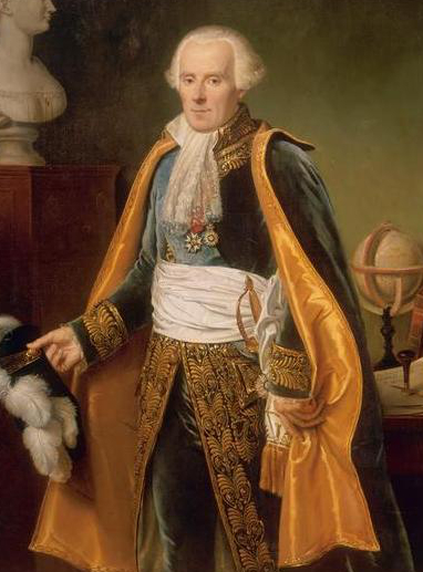
The foundations of probability have a long and interesting history (Hacking 2006; Todhunter 2014). The classical theory owes much to Pierre-Simon Laplace (1749–1827): see (Laplace 1825). However, a rigorous mathematical foundation for the theory was lacking, and was posed as part of one of David Hilbert’s (1862–1943) famous list of problems in 1900 (the 5th problem). After important work by Henri Lebesgue (1875–1941) and 'Emile Borel (1871–1956), it was Andrey Kolmogorov who succeeded in 1933 in providing the axioms that we use today (see the 1950 edition of his book (Kolmogorov 1950)). This approach declares that probabilities are measures.

A measure $\mu$ can be defined on any set $\Omega$ with a $\sigma$-algebra of subsets $\mathcal{F}$, and the defining axioms are versions of A1 and A4. The special property of a probability measure is just that $\mu(\Omega) = 1$. Measure theory is the theory that gives mathematical foundation to the concepts of length, area, and volume. For example, on $\mathbb{R}$ the unique measure that has $\mu (a,b) = b-a$ for intervals $(a,b)$ is the Lebesgue measure.

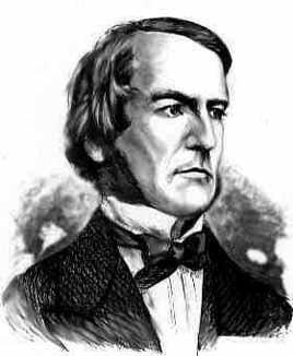
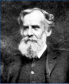
George Boole (1815–1864) and John Venn (1834–1923) both wrote books concerned with probability theory (Boole 1854), (Venn 1888); both were working before the formulation of Kolmogorov’s axioms.

As mentioned in Section 1.4, it is necessary in the general theory of probability to restricting events to some $\sigma$-algebra. The reason for this is that in standard ZFC set theory, when $\Omega$ is uncountable (such as $\Omega=[0,1]$ the unit interval), it follows from an argument by Vitali (1905) that many natural probability assessments, such as the continuous uniform distribution, cannot be modelled by a probability defined on all subsets of $\Omega$ satisfying A1–4: see for instance Chapter 1 of (Rosenthal 2007). In the case where $\Omega$ is countable, one can always define $\mathbb{P}$ on the whole of $2^\Omega$. In the case where $\Omega$ is uncountable, we usually do not explicitly mention $\Omega$ at all (when we work with continuous random variables, for example).

The formulation of the infinite coin-tossing experiment in Section 1.6 leads to the connection between coin tossing and the Lebesgue measure, as first described by Hugo Steinhaus in a 1923 paper.

An alternative approach to probability theory is to do away with axiom A4, in which case some of these technical issues can be avoided, at the expense of certain pathologies; however, in the standard approach to modern probability, based on measure theory, A4 is a central part of the theory.

Notation	We say (as sets)	We say (as events)	Meaning (as events)
\(A \cup B\)	\(A\) union \(B\)	\(A\) or \(B\)	\(A\) occurs or \(B\) occurs or both \(A\) and \(B\) occur
\(A \cap B\)	\(A\) intersect \(B\)	\(A\) and \(B\)	\(A\) occurs and \(B\) occurs
\(A^\mathrm{c} := \Omega \backslash A\)	\(A\) complement	not \(A\)	\(A\) does not occur
\(A\backslash B\)	\(A\) minus \(B\)	\(A\) but not \(B\)	\(A\) occurs but \(B\) does not
\(A\subseteq B\)	\(A\) is a subset of \(B\)	\(A\) implies \(B\)	if \(A\) occurs, then \(B\) must occur