$$ \newcommand{\pr}[1]{\mathbb{P}\left(#1\right)} \newcommand{\cpr}[2]{\mathbb{P}\left(#1\mid\,#2\right)} \newcommand{\expec}[1]{\mathbb{E}\left[#1\right]} \newcommand{\var}[1]{\text{Var}\left(#1\right)} \newcommand{\sd}[1]{\sigma\left(#1\right)} \newcommand{\cov}[1]{\text{Cov}\left(#1\right)} \newcommand{\cexpec}[2]{\mathbb{E}\left[#1 \vert#2 \right]} $$
5 Some applications of probability
5.1 Reliability of networks
Reliability theory concerns mathematical models of systems that are made up of individual components which may be faulty.
If components fail randomly, a key objective of the theory is to determine the probability that the system as a whole works. This will depend on the structure of the system (how the components are organized). This is an important problem in industrial (or other) applications, such as electronic systems, mechanical systems, or networks of roads, railways, telephone lines, and so on.
Once we know how to work out (or estimate) failure probabilities of these systems, we can start to ask more sophisticated questions, such as: How should the system be designed to minimize the failure probability, given certain practical constraints? What is a good inspection, servicing and maintenance policy to maximize the life of the system for a minimal cost?
In this course, to demonstrate an application of the probabilistic ideas we have covered so far, we address the basic question: Given a system made up of finitely many components, what is the probability that the system works? Whether the system functions depends on whether the components function, and on the configuration of those components.
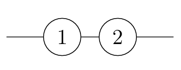
The system in (a) works if and only if both components 1 and 2 work.
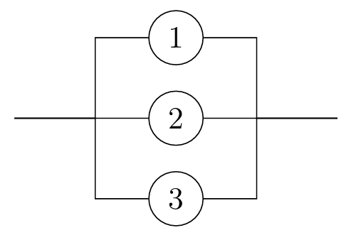
The system in (b) works if any of 1, 2, 3 work.
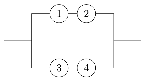
The system in (c) works if either both 1 and 2 work, or both 3 and 4 work (or all work).
Looking at reliability networks, and determining their reliability functions, is a source of lots of good examples to practice working with the axioms of probability (in particular A3, C1, and C6), as well as building up some more intuition about independence. Let’s have one more example (and there are a couple on the problem sheet, too).
5.2 Genetics
Inherited characteristics are determined by genes. The mechanism governing inheritance is random and so the laws of probability are crucial to understanding genetics.
Your cells contain 23 pairs of chromosomes, each containing many genes (while 23 pairs is specific to humans the idea is similar for all animals and plants). The genes take different forms called alleles and this is one reason why people differ (there are also environmental factors). Of the 23 pairs of chromosomes, 22 pairs are homologous (each of the pair has an allele for any gene located on this pair). People with different alleles are grouped by visible characteristics into phenotypes; often one allele, \(A\) say, is dominant and another, \(a\), is recessive in which case \(AA\) and \(Aa\) are of the same phenotype while \(aa\) is distinct. Sometimes, the recessive gene is rare and the corresponding phenotype is harmful, for example haemophilia or sickle-cell anaemia.
For instance, in certain types of mice, the gene for coat colour (a phenotype) has alleles \(B\) (black) or \(b\) (brown). \(B\) is dominant, so \(BB\) or \(Bb\) mice are black, while \(bb\) mice are brown with no difference between \(Bb\) and \(bB\).
With sickle-cell anaemia, allele \(A\) produces normal red blood cells but \(a\) produces deformed cells. Genotype \(aa\) is fatal but \(Aa\) provides protection against malarial infection (which is often fatal) and so allele \(a\) is common in some areas of high malaria risk.
To apply probability theory to the study of genetics, we use the basic principle of genetics: For each gene on a homologous chromosome, a child receives one allele from each parent, where each allele received is chosen independently and at random from each parent’s two alleles for that gene.
It is extremely important to note that genotypes of siblings are dependent unless we condition on parental genotypes. For example, if two black mice (which may each be BB or Bb) have 100 black offspring, you may conclude that the next offspring is overwhelmingly likely to also be black, because it is very likely that at least one parent is BB.
Genes can also affect reproductive fitness, as we see in the next example.
Things are slightly different for genes on the X or Y chromosomes (sex-linked genes).
These are the final chromosome pair, known as the sex chromosomes. Each may be X, a long chromosome, or Y, a short chromosome. Most of the genes on X do not occur on Y. Most people have sex determined as XX (female) or XY (male); YY is not possible.1
\(aa\) women are unhealthy;
\(a\) men are unhealthy;
otherwise the person is healthy.
A male child inherits his gene on the \(X\) chromosome from his mother (as he must get his \(Y\) from his father) with equal chance of the two alleles that the mother carries. A female child inherits her father’s single allele as well as one of her mother’s two alleles.
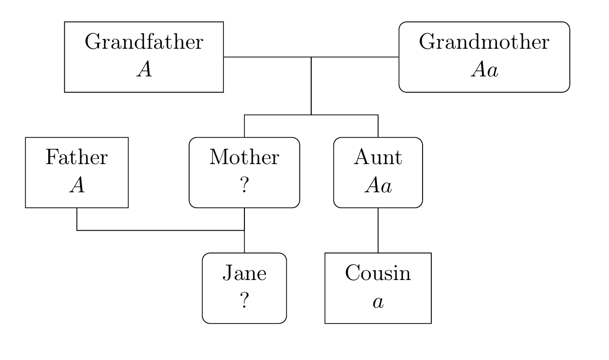
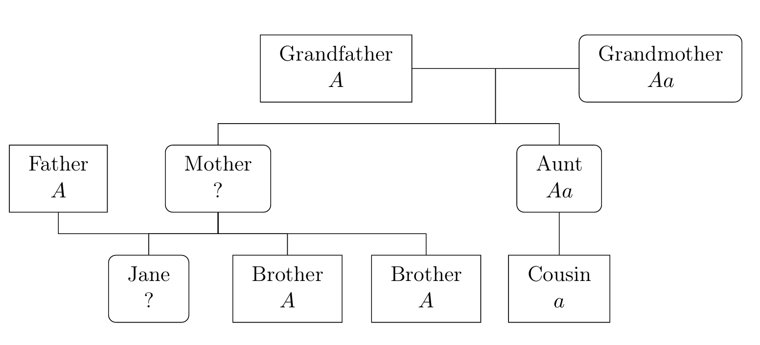
Jane is healthy. Her maternal aunt has an unhealthy son (Jane’s cousin). Jane’s maternal grandparents and her father are all healthy.
- What is the probability that Jane is genotype \(Aa\)?
Now suppose that Jane has two healthy brothers.
- What now is the probability that Jane is genotype \(Aa\)?
Answer: We start with part i. From the information given, we can add some information to the genetic tree. The healthy men are \(A\). A male child receives his single (X-carried) allele as a random selection from his mother’s two alleles (the genotype of his father has no bearing). Thus Jane’s Aunt must carry an \(a\). She cannot have inherited this from the healthy grandfather, so the grandmother must also carry an \(a\). This gives us the picture below.
Consider the events \(J = \{\text{Jane is $Aa$}\}\), \(M_1 = \{\text{mother is $AA$}\}\), and \(M_2 = \{\text{mother is $Aa$}\}\). From the tree above, we have \(M_1\) occurs if and only if Jane’s mother inherited an \(A\) from her mother, i.e., \(\pr{M_1} = 1/2\) and \(\pr{M_2} = 1/2\) too. Given the mother’s genotype, we can work out the probabilities for Jane’s inheritance. Thus, by the partition theorem, \[\begin{aligned} \pr{ J} & = \pr{ M_1} \cpr{J}{M_1} +\pr{M_2}\cpr{J}{M_2} \\ & = \frac{1}{2} \cdot 0 + \frac{1}{2} \cdot \frac{1}{2} = \frac{1}{4} .\end{aligned}\]
Now we move on to part ii. The tree is now augmented by the additional information about Jane’s siblings:
Let \(B= \{\text{Two brothers are } A\}\). We want \(\cpr{J}{B}\). Note that our knowledge of \(B\) changes our beliefs about the genotype of Jane’s mother. To see this more clearly, imagine that Jane had 100 brothers, all of whom were of type \(A\). Then we would be very nearly sure that Jane’s mother was of type \(AA\), and so Jane would be almost certainly of type \(AA\) too.
For the calculation, we use the partition theorem for conditional probabilities: \[\begin{aligned} \cpr{J}{B} & = \cpr{M_1}{B} \cpr{J}{M_1 \cap B} + \cpr{M_2}{B}\cpr{J}{M_2 \cap B} .\end{aligned}\] But given \(M_i\), \(J\) is independent of \(B\) so \[\begin{aligned} \cpr{J}{B} & = \cpr{M_1}{B} \cpr{J}{M_1} + \cpr{M_2}{B}\cpr{J}{M_2} .\end{aligned}\] As above, we have \(\cpr{J}{M_1} = 0\) and \(\cpr{J}{M_2} = 1/2\). By Bayes’s theorem, \[\begin{aligned} \cpr{M_2}{B} & = \frac{\cpr{B}{M_2}\pr{M_2}}{\cpr{B}{M_1}\pr{M_1}+\cpr{B}{M_2}\pr{M_2}} \\ & = \frac{ (1/2)^2 \cdot (1/2)}{1^2 (1/2) + (1/2)^2 \cdot (1/2)} = \frac{1}{5} .\end{aligned}\] So \[\cpr{J}{B} = 0 + \frac{1}{2} \cdot \frac{1}{5} = \frac{1}{10} .\] So seeing that Jane has two healthy brothers significantly reduces the chance that Jane is carrying an \(a\).
5.3 Hardy-Weinberg equilibrium
Consider a population of a large number of individuals evolving over successive generations. Consider a gene (on a homologous chromosome) with two alleles \(A\) and \(a\) and genotypes \(\{AA,Aa,aa\}\). Suppose the genotype proportions in the population (uniformly for males and females) at generation \(n = 0,1,2,\ldots\) are
| \(AA\) | \(Aa\) | \(aa\) |
|---|---|---|
| \(u_n\) | \(2v_n\) | \(w_n\) |
where we have \(u_n+2v_n+w_n = 1\). Suppose also that the proportions of the alleles in the population are
| \(A\) | \(a\) |
|---|---|
| \(p\) | \(q\) |
where \(p_n+q_n=1\). We see that \[p_n = \frac{2u_n +2v_n}{2u_n+4v_n+2w_n} = u_n + v_n\] and, similarly, \(q_n = v_n + w_n\).
Suppose that
the gene is neutral, meaning that different genotypes have equal reproductive success;
there is random mating with respect to this gene, meaning that each individual in generation \(n+1\) draws randomly two parents whose genotypes are independently in the proportions \(u_n\), \(2v_n\), \(w_n\).
How do the genotype proportions evolve over successive generations?
Consider the offspring of generation \(0\). Let \(FA\) = event that child gets allele \(A\) from father, \(MA\) = event that child gets allele \(A\) from mother, \(F_{AA}\) = event that father is \(AA\), \(F_{Aa}\) = event that father is \(Aa\), \(F_{aa}\) = event that father is \(aa\). Then \[\begin{aligned} \pr{FA} &= \pr{F_{AA}} \cpr{FA}{F_{AA}} +\pr{F_{Aa}} \cpr{FA}{F_{Aa}} +\pr{F_{aa}} \cpr{FA}{F_{aa}} \\ &= 1\cdot u_0 + \frac{1}{2}\cdot 2v_0 + 0 \cdot w_0 = u_0 +v_0 = p_0.\end{aligned}\] Similarly, \(\pr{MA} = p_0\). In particular, since parents contribute alleles independently, the probability distribution of the genotype of an individual in generation 1 is
| \(AA\) | \(Aa\) | \(aa\) |
|---|---|---|
| \(p_0^2\) | \(2p_0 (1-p_0)\) | \((1-p_0)^2\) |
Provided that the population is large enough (see the law of large numbers in Chapter 9) these will also be the generation 1 proportions of \(AA\), \(Aa\), \(aa\), i.e., \[u_1 = p_0^2, \qquad v_1 = p_0(1-p_0), \qquad w_1 = (1-p_0)^2 .\] Now let \(p_1 = u_1 + v_1\) be the proportion of \(A\) in the gene pool at generation 1. Substituting the values of \(u_1\), \(v_1\) we find that \[p_1 = u_1 + v_1 = p_0^2 + p_0(1-p_0) = p_0,\] i.e. the proportions of \(A\) and \(a\) in the gene pool are constant.
The same argument applies for later generations, so that \(p_n = p_0\) for all \(n\), i.e., the proportions of the two alleles in the gene pool remain constant. This means that, for \(n \geq 1\), \[u_n = p_0^2, \qquad v_n = p_0(1-p_0), \qquad w_n = (1-p_0)^2 ,\] so that the proportions of the three genotypes in the population remain constant in every generation after the first. This is called the Hardy–Weinberg equilibrium.
5.4 Historical context
Reliability for systems of infinitely many components is related to percolation.
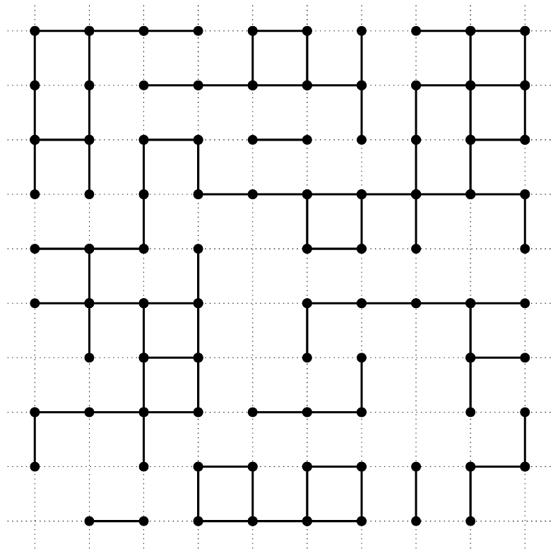
On the infinite square lattice \(\mathbb{Z}^2\), declare each vertex to be open, independently, with probability \(p \in [0,1]\), else it is closed. Consider the open cluster containing the origin, that is, the set of vertices that can be reached by nearest-neighbour steps from the origin using only open vertices. Percolation asks the question: for which values of \(p\) is the open cluster containing the origin infinite with positive probability? It turns out that for this model, the answer is: for all \(p > p_{\mathrm{c}}\) where \(p_{\mathrm{c}} \approx 0.593\).
The picture shows part of a percolation configuration, with open sites indicated by black dots and edges between open sites indicated by unbroken lines.
Percolation is an important example of a probability model that displays a phase transition. You may see more about it if you do later probability courses.
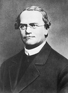
The laws governing the statistical nature of inheritance were first observed and formulated by monk Gregor Johann Mendel (1822–1884).
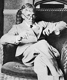
Biologist William Bateson (1861–1926)) coined the terms “genetics” and “allele”.
The Hardy of the Hardy–Weinberg law is G.H. Hardy (1877–1947), the famous mathematical analyst, who published it in 1908.
The statistician R.A. Fisher (1890–1962) made significant contributions to genetics, and much early work in statistics was concerned with genetical problems. A lot of this work contributed to a legacy of eugenics, which was used as a justification for racial discrimination.
The Wright–Fisher model formulates a random model for the evolution of genes in a population with mutation as an urn model (Mahmoud 2009, chap. 9).
The deep influence of probability theory on genetics has continued in recent times, with significant developments including the coalescent of J.F.C. Kingman.
X, XXX, XXY, and XYY can occur, but are very rare.↩︎