7  Multiple random variables

🥅 Goals

1. Understand a multivariate random variable as a function from the sample space to a higher dimensional space.

2. Understand jointly distributed discrete random variables:

• their joint probability mass function, marginal probability mass functions, and conditional probability mass functions.
• the partition theorem for discrete random variables.
• independence, and how to apply it.
• the properties of and links between the different probability mass functions, and how those properties and links arise from the axioms of probability distributions.

3. Understand continuously distributed random variables:

• their joint probability density function, marginal probability density functions, and conditional probability density functions.
• the partition theorem for jointly continuously distributed random variables.
• independence, and how to apply it.
• the properties of and links among the different probability density functions.

4. Understand how to work with functions of multiple random variables.

7.1 Joint probability distributions

It is essential for most useful applications of probability to have a theory which can handle many random variables simultaneously. To start, we consider having two random variables. The theory for more than two random variables is an obvious extension of the bivariate case covered below.

Remember that, formally, random variables are simply mappings from \(\Omega\) into some set. A bivariate random variable is a mapping from \(\Omega\) into a Cartesian product of two sets, i.e., a random variable whose values are ordered pairs of the form \((x,y)\). Of course, a bivariate random variable is a random variable according to our original definition, just with a special kind of set of possible values. However, the concept of bivariate random variable is a useful one if the individual components of the bivariate variable have their own meaning or interest.

Consider random variables \(X\) and \(Y\) defined on the same sample space \(\Omega\), \(X\colon\Omega\to X(\Omega)\) and \(Y\colon\Omega\to Y(\Omega)\). The mapping \((X,Y)\colon\Omega\to (X,Y)(\Omega)\) defined by \[(X,Y)(\omega):= (X(\omega),Y(\omega))\] is then a bivariate random variable.

Here is a picture:

Note that the set of possible values \((X,Y)(\Omega) = \{ ( X(\omega), Y(\omega) ) : \omega \in \Omega \}\) is a subset of the Cartesian product \(X(\Omega) \times Y(\Omega)\).

Example

On sample space \(\Omega = \{1,2,3,4,5,6\}\), define random variables \(X\) and \(Y\) by

\(\omega\)	1	2	3	4	5	6
\(X(\omega)\)	0	0	0	1	1	1
\(Y(\omega)\)	0	1	0	2	0	3

Then the bivariate random variable \((X,Y)\) is given by

\(\omega\)	1	2	3	4	5	6
\((X,Y)(\omega)\)	(0,0)	(0,1)	(0,0)	(1,2)	(1,0)	(1,3)

Note that \(X(\Omega) = \{0,1\}\), \(Y(\Omega) = \{0,1,2,3\}\), and \((X,Y)(\Omega) = \{ (0,0),(0,1),(1,0),(1,2),(1,3) \}\) which is a strict subset of \(\{0,1\} \times \{0,1,2,3\}\) (the outcome \((0,3)\) does not appear, for example).

Similarly to before, for any \(A \subseteq X(\Omega)\times Y(\Omega)\), we write ‘\((X,Y) \in A\)’ to denote the event \[\{ \omega \in \Omega\colon (X(\omega),Y(\omega)) \in A \}.\] For any \(x\in X(\Omega)\) and \(y\in Y(\Omega)\), we write ‘\(X = x,Y=y\)’ to mean the event \((X,Y)\in\{(x,y)\}\). We sometimes also write \(\{(X,Y)=(x,y)\}\) and \(\{(X,Y)\in A\}\) to emphasize that these are sets: \[\begin{aligned} \{X = x,Y=y\} &:= \{(X,Y)\in\{(x,y)\}\} \\ &= \{X=x\}\cap\{Y=y\} \\ &= \{\omega \in \Omega\colon X(\omega) = x\text{ and }Y(\omega)=y\}.\end{aligned}\] We may also write more complex expressions like: \[\{0\le X\le Y^2\le 1\}= \{ \omega \in \Omega\colon 0\le X(\omega)\le Y(\omega)^2\le 1 \}.\]

🔑 Key idea: Definition: Independence of two random variables

Two random variables \(X\) and \(Y\) on the same sample space \(\Omega\) are independent if \[\pr {X \in A, \, Y \in B } = \pr { X \in A } \pr {Y \in B} \text{ for all $A \subseteq X(\Omega)$ and $B \subseteq Y(\Omega)$.}\] In other words, \(X\) and \(Y\) are independent (as random variables) if and only if \(\{ X \in A \}\) and \(\{ Y \in B\}\) are independent as events for all sets \(A\) and \(B\).

Three random variables, \(X\), \(Y\), and \(Z\), say, are independent if the events \(\{ X \in A \}\), \(\{ Y \in B\}\), \(\{ Z \in C \}\) are mutually independent. Similarly for any finite collection of random variables. This definition is a bit unwieldy: it reduces to simpler statements in the cases of pairs of discrete or continuous random variables, which we look at next.

Advanced content

Later (when we talk about limit theorems such as the law of large numbers) we will need to talk about infinite sequences of independent random variables. A (possibly infinite) collection of random variables \(X_i\), \(i \in \mathcal{I}\), is independent if every finite nonempty sub-collection \(\mathcal{J} \subseteq \mathcal{I}\) is independent. In other words, \(X_i\), \(i \in \mathcal{I}\), are independent if for every finite \(\mathcal{J} \subseteq \mathcal{I}\), \[\pr{\bigcap_{j \in \mathcal{J}} \{ X_j \in A_j\} } = \prod_{j \in \mathcal{J}} \pr { X_j \in A_j } .\]

7.2 Jointly distributed discrete random variables

🔑 Key idea: Key definition: joint probability mass function

Let \((X,Y)\) be a bivariate discrete random variable with \(\pr{ (X,Y) \in \mathcal{Z}} =1\) for a finite or countable \(\mathcal{Z} \subseteq (X,Y)(\Omega)\). The joint probability mass function \(p(\cdot)\) of \(X\) and \(Y\) is defined by \[p(x, y):= \pr{X=x,Y=y} \qquad\text{ for all }(x,y) \in \mathcal{Z}.\]

Note there is nothing really new here, other than the terminology: this is just the definition of a discrete random variable written for the special case of a random variable \((X,Y)\) whose values are ordered pairs of the form \((x,y)\).

To avoid ambiguity, we sometimes write if \(p_{X,Y}(\cdot)\) if it is not clear from the context which random variables the two arguments refer to; note that \(p_{X,Y}(\cdot)\) is not the same as \(p_{Y,X}(\cdot)\).

It is the case that \((X,Y)\) is discrete if and only if the individual random variables \(X\) and \(Y\) are discrete. Proving this is the purpose of the following theorem, which and also explains how the marginal probability mass functions \(p(x)\) and \(p(y)\) of the individual random variables \(X\) and \(Y\) are connected to the joint probability mass function \(p(x,y)\). Note that it does no harm to take \(\mathcal{Z} = \mathcal{X} \times \mathcal{Y}\), extending the definition of \(p(x,y)\) with extra \(0\) values if necessary.

🔑 Key idea: Theorem: Joint and single discrete random variables

Let \(X\) and \(Y\) be two random variables on the same sample space \(\Omega\). Then the bivariate random variable \((X,Y)\) is discrete if and only if \(X\) and \(Y\) are both discrete. Moreover, if \(X\) and \(Y\) are both discrete with \(\pr {X \in \mathcal{X}} =\pr{Y \in \mathcal{Y}}=1\) for finite or countable \(\mathcal{X}\) and \(\mathcal{Y}\), then their marginal probability mass functions are given in terms of the joint probability mass function by \[\begin{aligned} p_X(x)&=\sum_{y\in \mathcal{Y}}p(x,y)\text{ for all }x\in \mathcal{X}, & p_Y(y)&=\sum_{x\in \mathcal{X}}p(x,y)\text{ for all }y\in \mathcal{Y}. \end{aligned}\]

Proof

First suppose that \(X\) and \(Y\) are discrete. Then there exist finite or countable sets of values \(\mathcal{X}\) and \(\mathcal{Y}\) such that \(\pr { X \in \mathcal{X} } =\pr{ Y \in \mathcal{Y} } =1\). Hence \(\pr {X \in \mathcal{X}, \, Y \in \mathcal{Y} } =1\). The bivariate random variable \((X,Y)\) thus has \(\pr { (X,Y) \in \mathcal{X} \times \mathcal{Y} } = 1\). Since \(\mathcal{X}\) and \(\mathcal{Y}\) are finite or countable, the Cartesian product \(\mathcal{X} \times \mathcal{Y}\) is also finite or countable. Hence \((X,Y)\) is discrete.

On the other hand, suppose that \((X,Y)\) is discrete. The possible values in \((X,Y)(\Omega)\) are ordered pairs of the form \((x,y)\), and there is a finite or countable set \(\mathcal{Z} \subseteq (X,Y)(\Omega)\) such that \(\pr { (X,Y) \in \mathcal{Z} } =1\). But if we set \(\mathcal{X} = \{ x : (x,y) \in \mathcal{Z}\}\) we have \(\pr { X \in \mathcal{X} } = \pr { (X,Y) \in \mathcal{Z} } = 1\), and \(\mathcal{X}\) is finite or countable (check this!), so \(X\) is discrete. Similarly for \(Y\). It remains to notice that, for example, with the same definition of \(\mathcal{X}\), \[\begin{aligned} \pr { Y = y} & = \pr { X \in \mathcal{X}, \, Y = y } \\ & = \pr{ \cup_{x \in \mathcal{X}} \{ X=x, \, Y = y \} }\\ & = \sum_{x \in \mathcal{X}} p(x,y) , \end{aligned}\] where we have used A4, the fact that \(\mathcal{X}\) is countable, and \(\pr{ X \in \mathcal{X} } =1\).

💪 Try it out

Roll two fair six-sided dice. Let \(X\) be the number of 6s rolled, and let \(Y\) be the number of 1s and 2s. Find the joint probability mass function \(p(x,y)\).

Answer:

The best way to present this is in a table:

\(p(x,y)\)	\(x=0\)	\(x=1\)	\(x=2\)
\(y=0\)	\(9/36\)	\(6/36\)	\(1/36\)
\(y=1\)	\(12/36\)	\(4/36\)	\(0\)
\(y=2\)	\(4/36\)	\(0\)	\(0\)

For example, \[\begin{aligned} p(0,0) & = \pr{\text{both scores in } \{3,4,5\}} = \frac{9}{36} ,\\ p(0,1) & = \pr{\text{first is } 1,2 \text{ and second } 3,4,5} + \pr{\text{first is } 3,4,5 \text{ and second } 1,2} \\ & = \frac{2 \cdot 3}{36} + \frac{3 \cdot 2}{36} = \frac{12}{36}, \end{aligned}\] and so on. Note that \(p(x,y)\) sums to 1!

Again, by C7, the joint probability mass function determines the joint probability distribution of \(X\) and \(Y\), and the values of the joint probability mass function sum to one:

Theorem: probability mass functions determine distributions for multiple random variables

Let \(X\) and \(Y\) be discrete random variables with \(\pr { (X,Y) \in \mathcal{Z} } =1\) for a finite or countable \(\mathcal{Z}\). Then we have that \[\pr{(X,Y)\in A} = \sum_{(x,y) \in A} p(x,y) \quad\text{ for all }A \subseteq \mathcal{Z}. \tag{7.1}\] In particular, \[\sum_{(x,y)\in \mathcal{Z} }p(x,y)=1.\]

This isn’t really a new idea: it is just the result about probability mass functions from Section 6.2 rewritten for the case of a discrete random variable whose possible values are ordered pairs \((x,y)\).

💪 Try it out

Continuing with the “two-dice” example, use \(p(x,y)\) to find \(\pr{ X \geq 1,\, Y \leq 1}\). Also, compute the marginal probability mass functions \(p_X(x)\) and \(p_Y(y)\).

Answer:

We have that \[\begin{aligned} \pr{ X \geq 1, \, Y \leq 1 } & = \pr { (X,Y) \in \{ (1,0), (1,1), (2,0), (2,1) \} } \\ & = p(1,0) + p(1,1) + p(2,0) + p(2,1) \\ & = \frac{6+4+1+0}{36} = \frac{11}{36} . \end{aligned}\] For the marginal distributions, we sum down columns and along rows in the table:

\(p(x,y)\)	\(x=0\)	\(x=1\)	\(x=2\)	\(p_Y(y)\)
\(y=0\)	\(9/36\)	\(6/36\)	\(1/36\)	\(16/36\)
\(y=1\)	\(12/36\)	\(4/36\)	\(0\)	\(16/36\)
\(y=2\)	\(4/36\)	\(0\)	\(0\)	\(4/36\)
\(p_X(x)\)	\(25/36\)	\(10/36\)	\(1/36\)	-

Note that this gives the same result as the binomial distribution, since \(X\sim\text{Bin}(2,1/6)\) and \(Y\sim\text{Bin}(2,1/3)\), so, for example, \[\pr{X=1} = \binom{2}{1} \cdot (1/6)^1 \cdot (5/6)^1 = \frac{10}{36} . \]

Examples

1. In a card game played with a standard 52 card deck, hearts are worth 1, the queen of spades is worth 13 and all other cards worth 0. Let \(X\), \(Y\) denote the values of the first and second cards dealt (without replacement, as usual). The possible outcomes of the bivariate random variable \((X,Y)\) are \[\{(0, 0),(1,0),(0, 1),(1, 1),(0, 13),(13, 0),(1, 13),(13, 1)\}\] (not \((13, 13)\)). With a well shuffled deck, the event \(A\) that the pair does not include the queen of spades, is \[\{ X \leq 1, Y \leq 1 \}=\{(X,Y)\in A\}\] where \[A=\{(0, 0),(1, 0),(0, 1),(1, 1)\}.\] So, by Equation 7.1, and a few counting arguments, \[\pr{(X,Y)\in A} =\frac{38}{52}\frac{37}{51} +\frac{1}{4}\frac{38}{51} +\frac{38}{52}\frac{13}{51} +\frac{1}{4}\frac{12}{51} = \frac{51 \times 50}{52\times 51} = \frac{50}{52}.\]

2. Discrete random variables \(X\) and \(Y\) are such that \(X\) takes possible values 0, 1, 2 while \(Y\) takes values 1, 2, 3, 4, and their joint distribution is given by

\(p(x,y)\)	\(y=1\)	\(y=2\)	\(y=3\)	\(y=4\)
\(x=0\)	0	0	0	1/4
\(x=1\)	0	1/4	1/4	0
\(x=2\)	1/4	0	0	0

From this table we can calculate \(\pr{X = x} = 1/4\), \(1/2\), \(1/4\) for \(x = 0\), 1, 2 respectively, i.e., \(X \sim \text{Bin}(2, 1/2)\). Similarly \(\pr{Y = y} = 1/4\) for \(y = 1\), 2, 3, 4 so \(Y\) is uniformly distributed on \(\{1, 2, 3, 4\}\).

Often we want to know the distribution of one random variable conditional on the value of another random variable.

Definition: Conditional probability mass function

Let \(X\) and \(Y\) be discrete random variables. For \(y \in \mathcal{Y}\), the conditional probability mass function of \(X\) given \(Y = y\) is defined by \[ p_{X \vert Y}(x,y) := \cpr{X=x}{Y=y}=\frac{p_{X,Y}(x,y)}{p_Y(y)} \] for all \(x\in \mathcal{X}\) and \(y\in \mathcal{Y}\) such that \(p_Y(y)>0\) and similarly, the conditional probability mass function of \(Y\) given \(X = x\) is \[ p_{Y \vert X}(y,x) := \cpr{Y=y}{X=x}=\frac{p_{X,Y}(x,y)}{p_X(x)} \] for all \(y\in \mathcal{Y}\) and \(x \in \mathcal{X}\) such that \(p_X(x)>0\).

There’s nothing new here, apart from the notation: this is just a particular case of the usual definition of conditional probability of one event given another, e.g., \[\cpr{X=x}{Y=y}=\frac{\pr{X=x, Y=y }}{\pr{Y=y}} = \frac{p_{X,Y}(x,y)}{p_Y(y)}.\]

💪 Try it out

Continuing from the “two dice” examples above, find \(p(x \vert y)\) and calculate the conditional probability \(\pr{X\ge 1\mid Y=0}\).

Answer:

Again, this is best presented in a table:

\(p_{X \vert Y}(x,y)\)	\(x=0\)	\(x=1\)	\(x=2\)
\(y=0\)	\(9/16\)	\(6/16\)	\(1/16\)
\(y=1\)	\(12/16\)	\(4/16\)	\(0\)
\(y=2\)	\(4/4\)	\(0\)	\(0\)

For example, \[ \begin{aligned} p_{X \vert Y}(0,2) & = \cpr{X=0}{Y=2} = \frac{\pr{X=0, Y=2}}{\pr{Y=2}} \\ & = \frac{p_{X,Y}(0,2)}{p_Y(2)} \\ & = \frac{4/36}{4/36} = 1. \end{aligned}\] Hence \[ \cpr{X\ge 1}{Y=0}=p_{X \vert Y}(1,0)+p_{X \vert Y}(2,0) =\frac{6}{16} + \frac{1}{16} = \frac{7}{16} . \]

There is also a version of P4 (partition theorem or, law of total probability) for discrete random variables; again, only the notation is new here.

Theorem: partition theorem for discrete random variables

Let \(X\) and \(Y\) be discrete random variables. Then, \[\begin{aligned} p_X(x) &= \sum_{y\in \mathcal{Y}} p_{X \vert Y}(x,y)p_Y(y). \end{aligned}\] Moreover, if \(X\) is real-valued, then for any functions \(g: \mathcal{Y} \to\mathbb{R}\) and \(h: \mathcal{Y} \to \mathbb{R}\) with \(g\leq h\), we can write \[\begin{aligned} \pr{g(Y)\le X\le h(Y)} &= \sum_{y\in \mathcal{Y}} \cpr{g(y)\le X\le h(y)}{Y=y} \pr{Y=y} \\ &= \sum_{y\in \mathcal{Y}} \sum_{x\in [g(y),h(y)]\cap \mathcal{X}} p_{X \vert Y}(x,y)p_Y(y). \end{aligned}\]

A version of the above result also holds with \(X\) and \(Y\) swapped.

Recall from the definition of independence of random variables that \(X\) and \(Y\) are independent random variables if events \(\{ X \in A \}\) and \(\{ Y \in B \}\) are independent for all \(A, B\). If \(X\) and \(Y\) are discrete, the following result gives a simpler characterization of independence.

🔑 Key idea: Lemma: Independence of discrete random variables

Two discrete random variables \(X\) and \(Y\) on the same sample space \(\Omega\) are independent if and only if \[p_{X,Y}(x,y)=p_X(x)p_Y(y) \text{ for all $x\in \mathcal{X}$ and $y\in \mathcal{Y}$.}\]

It follows that for independent discrete random variables \(X\) and \(Y\), \(p_{X \vert Y}(x,y)=p_X(x)\) whenever \(p_Y(y)>0\), and \(p_{Y \vert X}(y,x)=p_Y(y)\) whenever \(p_X(x)>0\).

Proof

By the definition of independence, we have that \[\pr { X= x, \, Y=y } = \pr { X=x} \pr {Y = y } ,\] as required. On the other hand, suppose that \(p_{X,Y}(x,y)=p_X(x)p_Y(y)\). Then by the “probability mass functions determine distributions for multiple random variables” theorem, for any sets \(A\) and \(B\), \[\begin{aligned} \pr{X \in A, Y \in B} & = \pr{ (X,Y) \in A \times B} = \sum_{x \in A} \sum_{y \in B} p_{X,Y}(x,y) \\ & = \sum_{x\in A} p_X(x) \sum_{y\in B} p_Y(y) \\ & = \pr{X \in A} \pr{Y \in B} , \end{aligned}\] so \(X\) and \(Y\) are independent.

💪 Try it out

Continuing the dice example, we saw that \(\pr{ X=2, Y=2} =0\) but \(\pr{X=2}\pr{Y=2}=\frac{1}{36} \cdot \frac{4}{36} \neq 0\). Hence \(X\) and \(Y\) are not independent. To show dependence it is enough to find a single pair \((x, y)\) where the joint probability mass function does not factorize. Conversely, to show independence it is necessary to consider all pairs \((x, y)\).

📖 Textbook references

If you want more help with this section, check out:

• Section 7.1 in (Blitzstein and Hwang 2019);
• or Chapter 6 in (Anderson, Seppäläinen, and Valkó 2018).

7.3 Jointly continuously distributed random variables

Definition: jointly continuous random variables

Consider two real-valued random variables \(X:\Omega\to\mathbb{R}\) and \(Y:\Omega\to\mathbb{R}\). We say that \(X\) and \(Y\) are jointly continuously distributed when there is a non-negative piecewise continuous function \(f(\cdot):\mathbb{R}^2\to\mathbb{R}\), called the joint probability density function, such that \[\pr{X\in [a,b], Y\in [c,d]} = \int_a^b \left(\int_c^d f(x,y)\, d y\right)\, d x\] for all \([a,b]\times [c,d]\subseteq\mathbb{R}^2\).

To avoid ambiguity we sometimes write \(f_{X,Y}(x,y)\) for the joint probability density of \(X\) and \(Y\). The interpretation of \(f(x,y)\) is that \[\pr{X\in [x,x+ \, d x], Y\in [y,y+ \, d y]}=f(x,y) \, d x \, d y \tag{7.2}\] for \(x,y\) at which \(f(x,y)\) is continuous.

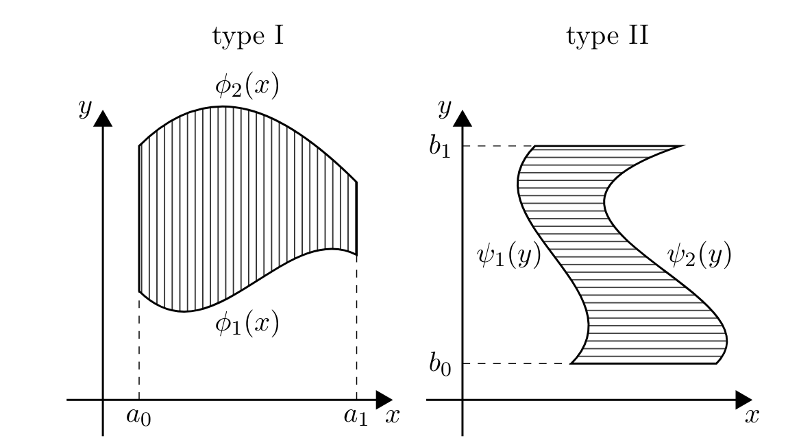
As before, the joint probability density function \(f(x,y)\) determines the joint probability \(\pr{(X,Y)\in A}\) for most events \(A\). More precisely, remember the definition of type I and II regions in the theory of multiple integration: a type I region is of the form \[D=\{a_0\leq x\leq a_1,\ \phi_1(x)\leq y \leq\phi_2(x)\}\] for some continuous functions \(\phi_1\) and \(\phi_2\), and a type II region is of the form \[D=\{\psi_1(y)\leq x\leq\psi_2(y),\ b_0\leq y\leq b_1\}\] for some continuous functions \(\psi_1\) and \(\psi_2\).

Regions of types 1 and 2

As we know from calculus, unions of regions of these types are precisely the regions over which we can integrate¹. So, we have:

Theorem: probabilities as integrals for joint distributions

If \(X\) and \(Y\) are jointly continuously distributed, then for any \(A\subseteq \mathbb{R}^2\) that is a finite union of type I and type II regions: \[\label{eq:defn:joint:pdf} \pr{(X,Y) \in A}=\iint\limits_A f(x,y)\, d x \, d y .\]

Again as before, \(f(x,y)\) integrates to one:

Corollary: joint densities integrate to 1

Let \(X\) and \(Y\) be jointly continuously distributed random variables. Then their joint probability density function integrates to one: \[\iint\limits_{\mathbb{R}^2}f(x,y) \, d x \, d y = 1.\]

💪 Try it out

Suppose that \(X\) and \(Y\) have joint probability density function \[f(x,y) = c(x^2 + y), \text{ for } -1 \leq x \leq 1, ~ 0 \leq y \leq 1 - x^2,\] with \(f(x,y) = 0\) otherwise. What is the value of \(c\)?

Answer: This is an exercise in multiple integration. We have from the Corollary that \[\begin{aligned} 1 & = \iint\limits_{\mathbb{R}^2}f(x,y) \, d x \, d y \\ & = \int_{-1}^1 \, d x \int_0^{1-x^2} c (x^2 + y) \, d y \\ & = c \int_{-1}^1 \, d x \left[ x^2 y + \frac{y^2}{2} \right]_0^{1-x^2} \\ & = \frac{c}{2} \int_{-1}^1 (1-x^4) \, d x \\ & = \frac{c}{2} \left[ x - \frac{x^5}{5} \right]_{-1}^1 \\ & = \frac{4}{5}c . \end{aligned}\] So we find that \(c = 5/4\).

💪 Try it out

Consider random variables \(X\) and \(Y\) with joint probability density function \[f(x,y) = \begin{cases} x + y & \text{if }(x, y) \in [0, 1]^2 \\ 0 & \text{otherwise}. \end{cases}\]

1. Calculate \(\pr{1/4 < X < 3/4, 0 < Y < 1/2}\)

2. Calculate \(\pr{X^2 < Y < X}\)

Answer:

Again, this is an exercise in multiple integration. For part (a) we have \[\begin{aligned} \pr{1/4 < X < 3/4, 0 < Y < 1/2} & = \int_{1/4}^{3/4} \, d x \int_{0}^{1/2} (x+y) \, d y \\ & = \int_{1/4}^{3/4} \, d x \left[ xy + \frac{y^2}{2} \right]_0^{1/2} \\ & = \int_{1/4}^{3/4} \left( \frac{x}{2} + \frac{1}{8} \right) \, d x \\ & = \frac{3}{16} . \end{aligned}\] For part (b), we have \[\begin{aligned} \pr{X^2 < Y < X} & = \int_0^1 \, d x \int_{x^2}{x} (x+y) \, d y = \int_{0}^{1} \, d x \left[ xy + \frac{y^2}{2} \right]_{x^2}^{x}\\ & = \int_0^1 \left( \frac{3x^2}{2} - x^3 - \frac{x^4}{4} \right) \, d x = \frac{3}{20} . \end{aligned}\]

Note that, if \(X\) and \(Y\) are jointly continuously distributed, then for any interval \([a,b]\), \[\pr{X\in [a,b]} = \pr{X\in [a,b], Y\in\mathbb{R}} = \int_a^b\left(\int_{-\infty}^\infty f(x,y) \, d y \right) \, d x,\] so, by the definition of a continuous random variable, \(X\) is continuously distributed as well, as is \(Y\) by a similar argument. We have shown the following:

Corollary

Let \(X\) and \(Y\) be jointly continuously distributed random variables. Then \(X\) and \(Y\) are (each separately) continuously distributed, with \[\begin{aligned} f_X(x) = \int_{-\infty}^\infty f(x,y) \, d y, \text{ for all }x\in\mathbb{R}, \qquad f_Y(y) = \int_{-\infty}^\infty f(x,y) \, d x, \text{ for all }y\in\mathbb{R}. \end{aligned}\]

In a multivariate context, the probability density functions \(f_X(x)\) and \(f_Y(y)\) are also called marginal probability density functions.

💪 Try it out

Continuing from the previous example, we have that for \(x \in [0,1]\), \[f_X(x) = \int_0^1 (x+y) \, d y = \left[ xy + \frac{y^2}{2} \right]_0^1 = x + \frac{1}{2} ,\] so \[f_X(x) = \begin{cases} x + \frac{1}{2} & \text{if } 0 \leq x \leq 1,\\ 0 & \text{otherwise} .\end{cases} \]

💪 Try it out

As in a previous example, suppose that \(X\) and \(Y\) have joint probability density function \[f(x,y) = c(x^2 + y), \text{ for } -1 \leq x \leq 1, ~ 0 \leq y \leq 1 - x^2,\] with \(f(x,y) = 0\) otherwise. we find \[f_(x) = \frac{5}{4} \int_0^{1-x^2} (x^2 + y)\ dy = \frac{5}{8}(1 - x^4)\] for \(-1 \leq x \leq 1\) and 0 otherwise; \[f_(y) = \frac{5}{4} \int_{-\sqrt{1-y}}^{\sqrt{1-y}} (x^2 + y) \, d x = \frac{5}{6}(1 + 2y) \sqrt{1 - y}\] for \(0 \leq y \leq 1\) and 0 otherwise.

Advanced content

So, if \(X\) and \(Y\) are jointly continuously distributed, then both \(X\) and \(Y\) are also continuously distributed separately. Unlike the discrete case (the “joint and single discrete random variables” theorem), the converse, however, is not true in general, as the following example shows.

Example

Let \(X\) be a continuously distributed random variable, and let \(Y:= 2X\). Then both \(X\) and \(Y\) are continuously distributed separately, however \(X\) and \(Y\) are not jointly continuously distributed. Indeed, suppose that \(X\) and \(Y\) were jointly continuously distributed with density function \(f(x,y)\). Then, with \(A=\{(x,y): 2x=y\}\), \[\iint\limits_A f(x,y) \, d x \, d y = \int_{-\infty}^{+\infty}\left(\int_{2x}^{2x} f(x,y) \, d y\right)\, d x = 0.\] This implies that \(\pr{2X=Y}=0\) for every two jointly continuously distributed random variables \(X\) and \(Y\). But, because for our choice of \(X\) and \(Y\), obviously \(\pr{2X=Y}=1\); so, by contradiction, \(X\) and \(Y\) cannot be jointly continuously distributed.

Conditional probability density function

Let \(X\) and \(Y\) be jointly continuously distributed random variables. The conditional probability density function of \(X\) at \(Y=y\) is defined by \[f_{X\vert Y}(x \vert y):= \frac{f_{X,Y}(x,y)}{f_Y(y)} \quad \text{ for all }x,y\in\mathbb{R}\text{ such that }f_Y(y) > 0.\] and similarly, the conditional probability density function of \(Y\) at \(X=x\) is \[f_{Y\vert X}(y \vert x):= \frac{f_{X,Y}(x,y)}{f_X(x)} \quad \text{ for all }x,y\in\mathbb{R}\text{ such that }f_X(x) > 0.\]

Advanced content

Roughly speaking, \(f_{X\vert Y}(x \vert y)\) should be thought of as the probability density function of \(X\) conditional on \(Y=y\). Because the event \(Y=y\) has probability \(0\), this interpretation needs a bit of work to realize rigorously. A formal manipulation using Equation 6.2 and Equation 7.2 goes as follows: \[\begin{aligned} \cpr{X\in[x,x+ \, d x]}{Y\in[y,y+ \, d y]} &= \frac{\pr{X\in[x,x+ \, d x],Y\in[y,y+ \, d y]}}{\pr{Y\in[y,y+\, d y]}} \\ &= \frac{f_{X,Y}(x,y)\, d x \, d y}{f_Y(y)\, d y} = f_{X\vert Y}(x \vert y)\, d x, \end{aligned}\] so \(f_{X\vert Y}(x \vert y)\) is the probability density of \(X\) conditional on \(Y\in[y,y+\, d y]\). This relies on \(f_{X,Y}\) and \(f_Y\) being continuous so that Equation 6.2 and Equation 7.2 are valid.

Theorem: Partition theorem for jointly continuous random variables

Let \(X\) and \(Y\) be jointly continuously distributed random variables. Then, \[f_X(x) = \int_{-\infty}^{+\infty} f_{X|Y}(x \vert y)f_Y(y)\, d y.\] Moreover, for any piecewise continuous functions \(g:\mathbb{R}\to\mathbb{R}\) and \(h:\mathbb{R}\to\mathbb{R}\) with \(g\le h\), we can write, \[\begin{aligned} \pr{g(Y)\le X\le h(Y)} &= \int_{-\infty}^{+\infty} \left( \int_{g(y)}^{h(y)} f(x \vert y)\, d x \right) f_(y)\, d y. \end{aligned} \tag{7.3}\]

Advanced content

We can formulate this theorem in a way that is more similar to the discrete case. For any event \(A\), and any continuously distributed random variable \(Y\), we define \[\cpr{A}{Y=y}:= \lim_{h\to 0}\pr{A\mid Y\in [y,y+h]}\] whenever \(\pr{A\mid Y\in [y,y+h]}>0\) for all \(h\) sufficiently small—this happens when \(f_(y)\) is continuous at \(y\) and \(f_(y)>0\). Our usual definition of conditional probability does not apply, because \(\pr{Y=y}=0\), so \(\cpr{A}{Y=y}\) is not really a conditional probability. One should be warned that the notation \(\cpr{A}{Y=y}\) for continuously distributed \(Y\) can lead to extremely confusing issues, such as Borel’s paradox. Anyway, ignoring potential pitfalls, with this notation \[\cpr{g(y)\le X\le h(y)}{Y=y} = \int_{g(y)}^{h(y)}f(x \vert y) \, d x,\] and consequently, we can rewrite Equation 7.3 as \[\begin{aligned} \pr{g(Y)\le X\le h(Y)} &= \int_{-\infty}^{+\infty} \cpr{g(y)\le X\le h(y)}{Y=y}f(y)\, d y. \end{aligned}\]

Similarly to the discrete case, independence can be characterized as a factorization property of the joint probability density function.

🔑 Key idea: Lemma: independence of jointly continuous random variables

Two jointly continuously distributed random variables \(X\) and \(Y\) are independent if and only if \[f_{X,Y}(x,y)=f_X(x)f_Y(y) \text{ for all $x$ and $y\in\mathbb{R}$.}\]

For independent jointly continuously distributed \(X\) and \(Y\), \(f_{X\vert Y}(x \vert y)=f_X(x)\) whenever \(f_Y(y)>0\), and \(f_{Y\vert X}(y \vert x)=f_Y(y)\) whenever \(f_X(x)>0\).

Example

Suppose \(X\) and \(Y\) have joint probability density function \[f(x,y) = \begin{cases} 3e^{-(x+3y)} & \text{if } x\ge 0\text{ and }y\ge 0, \\ 0 & \text{otherwise}. \end{cases}\] Because we can write \(f(x,y)\) as \(e^{-x}\cdot 3e^{-3y}\) (for \(x\ge 0\) and \(y\ge 0\)), it follows that \(X \sim \mathcal{E}(1)\) and \(Y \sim \mathcal{E}(3)\), and they are independent. We can calculate things like, for \(a>0\), \[\begin{aligned} \pr{aY < X} &= \int_0^\infty \left(\int_{ay}^{\infty} f(x \vert y) \, d x\right) f_(y)\, d y \\ &= \int_0^\infty \left(\int_{ay}^{\infty} e^{-x}\, d x\right) 3e^{-3y}\, d y = \int_0^\infty e^{-ay}\cdot 3e^{-3y}\, d y = 3/(3+a). \end{aligned}\]

📖 Textbook references

If you want more help on this section, check out:

• Section 7.1 in (Blitzstein and Hwang 2019);
• Section 6.2 in (Anderson, Seppäläinen, and Valkó 2018);
• or Sections 8.1 and 8.3 in (Stirzaker 2003).

7.4 Functions of multiple random variables

Suppose \(X:\Omega\to X(\Omega)\) and \(Y:\Omega\to Y(\Omega)\) are (discrete or continuous) random variables, and \(g: X(\Omega)\times Y(\Omega)\to\mathcal{S}\) is some function assigning a value \(g(x,y) \in \mathcal{S}\) to each point \((x,y)\). Then \(g(X,Y)\) is also a random variable, namely the outcome to a ‘new experiment’ obtained by running the ‘old experiments’ to produce values \(x\) for \(X\) and \(y\) for \(Y\), and then evaluating \(g(x,y)\).

\(g(X,Y)\) as a random variable

Formally, \(g(X,Y):= g\circ (X,Y)\), or in more specific terms, the random variable \(g(X,Y):\Omega\to\mathcal{S}\) is defined by: \[g(X,Y)(\omega):= g(X(\omega),Y(\omega))\text{ for all }\omega\in\Omega.\] For example: \[\pr{ g(X,Y)\in A } = \pr{ \{\omega\in\Omega: g(X(\omega),Y(\omega))\in A\} } \text{ for all } A\subseteq\mathcal{S}.\]

For any random variables \(X\) and \(Y\), \(X+Y\), \(X - Y\), \(XY\), \(\min(X, Y)\), \(e^{t(X + Y)}\), and so on, are all random variables as well.

💪 Try it out

Consider the jointly continuous random variables \(X\) and \(Y\) from . Define a new random variable \(S = X+Y\).

1. Calculate \(F_S(\cdot)\) and hence deduce that \(S\) is a continuous random variable.

2. Identify \(f_S\).

Answer:

For part (a), we note that \(\pr{ 0 \leq S \leq 2} = 1\) so \(F_S(s) =0\) for \(s <0\) and \(F_S(s) =1\) for \(s \geq 2\). Suppose that \(0 \leq s \leq 1\). Then \[\begin{aligned} F_S(s) & = \pr{ X+Y \leq s } = \int_0^s \left(\int_0^{s-y}(x+y) \, d x\right) \, d y \\ &= \int_0^s \left[x^2/2+xy\right]_{x=0}^{x=s-y} \, d y \\ &= \frac{1}{2} \int_0^s (s^2 - y^2) \, d y \\ & =\frac{s^3}{3} . \end{aligned}\] Next, for \(1 < s \leq 2\), \[\begin{aligned} F_S(s) & = \pr { X+Y \leq s } \\ & = \int_0^{s-1}\left(\int_0^1 (x+y) \, d x\right) \, d y + \int_{s-1}^1\left(\int_0^{s-y} (x+y) \, d x\right) \, d y \\ & = \int_0^{s-1} (y + 1/2) \, d y + \frac{1}{2} \int_{s-1}^1 (s^2 - y^2) \, d y \\ & = s^2 - \frac{1 + s^3}{3}. \end{aligned}\] We see that \(F_S(\cdot)\) is continuous, and piecewise differentiable. Hence there is a density which is obtained by differentiation: \[f_S(s) =\frac{\, d F_S(s)}{\, d s} = \begin{cases} s^2 &\text{if }0 \le s \le 1, \\ 2s - s^2 & \text{if }1 < s \le 2, \\ 0 &\text{elsewhere}, \end{cases}\] and in fact \(f_S(s)\) is continuous everywhere.

📖 Textbook references

If you want more help on this section, check out:

• Section 3.9 in (DeGroot and Schervish 2013).

Anderson, D. F., T. Seppäläinen, and B. Valkó. 2018. Introduction to Probability. Cambridge University Press.

Blitzstein, J. K., and J. Hwang. 2019. Introduction to Probability. Texts in Statistical Science Series. CRC Press.

DeGroot, M. H., and M. J. Schervish. 2013. Probability and Statistics. 4th ed. Harlow, England: Pearson.

Stirzaker, D. 2003. Elementary Probability. Second. Cambridge University Press.

---

1. At least when restricted to the Riemann integral.