9 Limit theorems

🥅 Goals

Understand and know how to prove the weak law of large numbers, for proportions as well as for general random variables, and know under what conditions the weak law applies.
Understand and know how to prove (by means of moment generating functions) the central limit theorem.
Know under what conditions the central limit theorem applies.
Know how to exploit the central limit theorem to approximate the binomial distribution, and under what circumstances.
Know the definition and properties of moment generating functions.
Know how to derive the moment generating function of a given distribution.

9.1 The weak law of large numbers

The results of this section describe limiting properties of distributions of sums of random variables using only some assumptions about means and variances.

Toss a coin $n$ times, where the probability of heads is $p$, independently on each toss. Let $X$ be the number of heads and let $B_n:= X/n$ be the proportion of heads in the $n$ tosses. Then, because $X\sim\text{Binom}(n,p)$ has expectation $np$ and variance $np(1-p)$, \[\begin{aligned} \expec{B_n} &= \expec{X}/n = p, & \var{B_n} &= \var{X}/n^2 = p(1-p)/n. \end{aligned}\]

So, by Chebyshev’s inequality, for any $\epsilon>0$, \[\pr{|B_n - p| \geq \epsilon} \leq \frac{p(1-p)}{n\epsilon^2}.\] Whence, \[\pr{|B_n - p| \geq \epsilon}\to 0 \text{ as } n \to \infty,\] no matter how small $\epsilon$ is. In other words, as $n \rightarrow \infty$, the sample proportion is with very high probability within any tiny interval centred on $p$.

The same argument applies more generally.

🔑 Key idea: Theorem: the weak law of large numbers

Suppose we have an infinite sequence $X_1$, $X_2$, … of independent random variables with the same mean and variance: \[\begin{aligned} \expec{X_i} = \mu \text{ and } \var{X_i} = \sigma^2 \text{ for all } i. \end{aligned}\] Consider the sample average $\bar{X}_n := \frac{1}{n}\sum_{i=1}^n X_i$. Then, for any $\epsilon>0$, \[ \lim_{n\to\infty}\pr{ | \bar{X}_n - \mu | > \epsilon } = 0. \tag{9.1}\]

In other words, the sample average has a very high probability of being very near the expected value $\mu$ when $n$ is large. The type of convergence in Equation 9.1 is called convergence in probability: the weak law of large numbers says that “$\bar{X}_n$ converges in probability to $\mu$”.

Proof

We use Chebyshev’s inequality to bound the probability that we are trying to show is small.

First note that, by linearity of expectation, $\expec{\bar{X}_n}=\frac{1}{n} \sum_{i=1}\expec{X_i}=\mu$ and, by independence, $\var{\bar{X}_n}= \frac{1}{n^2} \sum_{i=1}^n \var{X_i} = \frac{\sigma^2}{n}$. So, by Chebyshev’s inequality, \[P\bigl( |\bar{X}_n - \mu| \geq \epsilon \bigr) \leq \frac{\sigma^2}{n\epsilon^2},\] which indeed converges to zero as $n$ tends to infinity.

Advanced content

The assumption of finite variances in this theorem is not necessary. The weak law of large numbers holds assuming only that $\expec{X_i} = \mu$ for independent $X_i$: for this and other more advanced results, see (Feller 1968, chap. 10).

Examples

Measure the heights $H_i$ of $n$ randomly selected people from a very large population, where $\mu$, $\sigma^2$ are the average and the variance of heights over the whole population.

Then $\expec{H_i} = \mu$, $\var{H_i} = \sigma^2$ and so, as long as the collection of heights is not too asymmetric, the chance of the average height $\bar{X}_n$ being more than a small amount from $\mu$ is very small; i.e. almost all large samples have average near $\mu$.
Here is an application to repeated sampling. Let $X$ be a random variable whose distribution we want to study by ‘sampling’, i.e., observing a number of independent random variables $X_1, X_2, \ldots, X_n$ which all have the same distribution as $X$. We could observe $X_1,X_2,\ldots, X_n$ and consider \[\pi_n (a,b ) = \frac{1}{n} \sum_{i=1}^n 𝟙 \{ X_i \in [a,b) \} ,\] the proportion of observations whose value falls in the interval $[a,b)$. Since the $X_i$ are independent, so are the indicator random variables, and we know that $\expec{ 𝟙 \{ X_i \in [a,b) \} } = \pr { X_i \in [a,b) }$. So the law of large numbers says that $\pi_n (a,b)$ will approach $\pr { X_i \in [a,b) }$ for large $n$ with high probability. Another way to see this is to observe that $\sum_{i=1}^n 𝟙 \{ X_i \in [a,b) \}$ is a binomial random variable.

If we want to look at the distribution of $X$, we would construct a histogram using the proportions $\pi_n (a_i,b_i )$ over a collection of ‘bins’ $[a_i,b_i)$. If there are only finitely many bins, then it follows that all the $\pi_n$’s tend to be close to their respective probabilities. For example, the picture in Figure 9.1 shows a histogram produced by $10^4$ simulations of a $U(0,1)$ random variable: the fact that the histogram is a good approximation to the probability density function can, in this instance, be seen as a consequence of the law of large numbers.

Figure 9.1: Histogram generated from $10^4$ simulations of a $\text{U}(0, 1)$ random variable. The vertical axis is the frequency.

📖 Textbook references

If you want more help with this section, check out:

Section 10.2 in (Blitzstein and Hwang 2019);
Section 9.2 in (Anderson, Seppäläinen, and Valkó 2018);
or Section 5.8 in (Stirzaker 2003).

9.2 The central limit theorem

If the law of large numbers is a ‘first order’ result, a ‘second order result’ is the famous central limit theorem, which describes fluctuations around the law of large numbers, and explains, in part, why the normal distribution has a central role in statistics. A sequence of random variables $X_1, X_2, \ldots$ are independent and identically distributed (i.i.d. for short) if they are mutually independent and all have the same (marginal) distribution.

🔑 Key idea: Theorem: the Central Limit Theorem

Suppose we have a sequence $X_1$, $X_2$, …of i.i.d. random variables. Let \[\begin{aligned} \mu&:= \expec{X_i} \text{ and } \sigma^2&:=\var{X_i} , \end{aligned}\] with $\sigma>0$. Let $S_n:=\sum_{i=1}^n X_i$, $\bar{X}_n:= S_n/n$, and \[Z_n :=\frac{S_n-n \mu}{\sigma \sqrt{n}} =\frac{\bar{X}_n- \mu}{\sigma/\sqrt{n}}\] Then, for any $z\in\mathbb{R}$, \[\lim_{n\to\infty} F_{Z_n}(z) = \lim_{n\to\infty} \pr{Z_n \leq z}=\Phi(z).\] We say that $Z_n$ converges in distribution to the standard normal distribution.

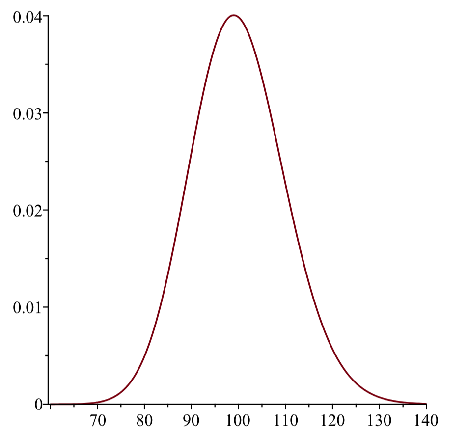
In other words, for large $n$, we have that approximately $Z_n \approx \mathcal{N}(0,1)$. Note that the definition of $Z_n$ is such that $\expec{Z_n} =0$ and $\var{Z_n}=1$. The content of the central limit theorem is that it should be approximately normal. Consequently, if we also invoke , we approximately have that $S_n \approx \mathcal{N}(n\mu,n\sigma^2)$ and $\bar{X}_n \approx \mathcal{N}(\mu, \sigma^2/n)$, i.e., typical values of $S_n$ are of order $\sigma\sqrt{n}$ from $n\mu$ while typical values of $\bar{X}_n$ are of order $\sigma/\sqrt{n}$ from $\mu$. In other words, for large enough $n$, by , \[\begin{aligned} \pr{S_n \leq x} &\approx \Phi\left(\frac{x-n\mu}{\sigma\sqrt{n}}\right), \\ \pr{\bar{X}_n \leq x} &\approx \Phi\left(\frac{x-\mu}{\sigma/\sqrt{n}}\right). \end{aligned}\]

Example

Suppose $X_1, X_2, \ldots$ are i.i.d. exponential random variables with parameter 1, i.e., they have probability density function $f(x) = e^{-x}$ for $x>0$ and $f(x) =0$ otherwise.

Consider $S_n = \sum_{i=1}^n X_i$. The central limit theorem says that $S_n$ will be approximately normal for large $n$, and since we know $\expec { X_i } =1$ and $\var { X_i} =1$ in this case, $S_n$ will be approximately $\mathcal{N}(n,n)$ for large $n$.

How “large” should $n$ be? Well, in this case it turns out we can compute the distribution of $S_n$ exactly. It is an example of a gamma distribution, and for $n \geq 1$, $S_n$ has probability density function \[f_n (x) = \begin{cases} \dfrac{e^{-x} x^{n-1}}{(n-1)!} & \text{if } x > 0, \\ 0 & \text{elsewhere}. \end{cases}\] See Figure 9.2 for some plots of this for various values of $n$.

Advanced content

The conditions of the central limit theorem can be substantially weakened.

The assumption that the $X_i$ are identically distributed can be dropped and replaced with the Lindeberg condition: see e.g. (Feller 1971, chap. VIII).

In fact, the random variables $X_1$, $X_2$,… need be neither identical nor independent: it is sufficient that we can turn them into a normalized martingale. Without going into too much detail, it suffices to assume that \[\begin{aligned} \cexpec{X_{n+1}}{X_1=x_1\dots X_n=x_n}&=\expec{X_{n+1}} \\ \var{X_{n+1} \vert X_1=x_1\dots X_n=x_n}&=\var{X_{n+1}}>0 \end{aligned}\] for all $n$ and all possible values for $x_1$, …,$x_n$. In this case, the sequence of random variables \[Z_n:=\frac{\sum_{k=1}^n(X_{k}-\expec{X_{k}})}{\sqrt{\sum_{k=1}^n \var{X_{k}}}}\] converges to a $\mathcal{N}(0,1)$ random variable whenever the martingale version of the Lindeberg condition is satisfied. For further details, see for instance (Nelson 1987, chap. 14 & 18).

💪 Try it out

Potatoes with an average weight of 100g and standard deviation of 40g are packed into bags to contain at least 2500g. What is the chance that more than 30 potatoes will be needed to fill a given bag?

Answer:

Let $N$ be the number needed to exceed 2500 and $W$ be the total weight of 30 potatoes, $W= \sum_{i=1}^{30} X_i$. Then $\expec{W} = 30 \cdot 100 = 3000$ and $\var{W} = 30 \cdot 40^2 = 48000$, and the central limit theorem says that \[\frac{W - 3000}{\sqrt{48000}} \approx \mathcal{N} (0,1) .\] Also, $\{N > 30\} = \{W < 2500\}$ and so \[\begin{aligned} \pr { N > 30 } & = \pr{W < 2500} \\ & = \pr { \frac{W-3000}{\sqrt{48000}} < \frac{2500-3000}{\sqrt{48000}} } \\ & \approx \pr { Z < -2.282 }, \end{aligned}\] where $Z\sim\mathcal{N}(0,1)$. From the tables, this probability is \[\pr { Z < -2.282 } = \pr { Z > 2.282 } = 1 - \Phi (2.282) \approx 0.011. \]

💪 Try it out

Measurements from a particular experiment have mean $\mu$ (unknown) and known standard deviation $\sigma = 2.5$. We perform 20 repetitions of the experiment and use $\bar{X}_{20}$ to estimate $\mu$. What is $\pr{ | \bar{X}_{20} - \mu | < 1 }$?

Answer:

The central limit theorem says that \[\frac{\bar{X}_n - \mu}{\sqrt{ 2.5^2 /n }} \approx \mathcal{N}(0,1) .\] So \[\begin{aligned} \pr { | \bar{X}_{20} - \mu | <1 } & = \pr { -1 \leq \bar{X}_{20} - \mu \leq 1 }\\ & = \pr { -\frac{1}{\sqrt{ 2.5^2/20}} \leq \frac{\bar{X}_{20} - \mu}{\sqrt{ 2.5^2 / 20 }} \leq \frac{1}{\sqrt{ 2.5^2/20}} } \\ & \approx \pr { -1.789 \leq Z \leq 1.789 } , \end{aligned}\] where $Z\sim\mathcal{N}(0,1)$. Thus \[\begin{aligned} \pr { | \bar{X}_{20} - \mu | <1 } & \approx \Phi (1.789) - \Phi (-1.789)\\ & = 2 \Phi (1.789) -1\\ & \approx 0.92 , \end{aligned}\] using normal tables.

Note that Chebyshev’s inequality gives the weaker result \[\begin{aligned} \pr{ | \bar{X}_{20} - \mu | < 1 } & = 1 - \pr{ | \bar{X}_{20} - \mu | \geq 1 } \\ & \geq 1 - \frac{\var{\bar{X}_{20}}}{1^2} \\ & = 1 -\frac{2.5^2}{20} \approx 0.69 . \end{aligned}\]

Remember that we can write any binomially distributed random variable as a sum of independent Bernoulli random variables. Consequently:

Corollary: Normal approximation to the Binomial

Let $X\sim\text{Bin}(n, p)$ with $0<p<1$, $B_n:= X/n$, and \[Z_n:= \frac{X - np}{\sqrt{np(1-p)}} = \frac{B_n - p}{\sqrt{p(1-p)/n}}\] Then \[\lim_{n\to\infty}F_{Z_n}(z) = \lim_{n\to\infty}\pr{Z_n\le z}=\Phi(z).\]

This means that, when $X\sim\text{Bin}(n,p)$ with $0<p<1$ and large enough $n$, then for any $x\in\mathbb{R}$, we approximately have that \[\pr{X \leq x} \approx\Phi\left( \frac{x-np}{\sqrt{np(1-p)}} \right)\] For moderate $n$, a continuity correction improves the approximation; e.g. for $k\in\mathbb{N}$: \[\begin{aligned} \pr{X \leq k}&=\pr{X\leq k+0.5} \approx \Phi\left( \frac{k+0.5-\mu}{\sigma} \right) \\ \pr{k\le X}&=\pr{k-0.5\le X} \approx 1-\Phi\left( \frac{k-0.5-\mu}{\sigma} \right) \end{aligned}\]

💪 Try it out

Consider a multiple choice test with 50 questions, one mark for each correct answer. Independently for each question, a particular student has chance $1/2$ of answering correctly. Find, approximately, the probability of the student scoring at least 30 marks.

Answer

Let $X$ = student’s score, so $X \sim \text{Bin}(50, 1/2)$. Then $\expec{X} = 50/2 =25$ and $\var{X} = 50/4 = 25/2$. The normal approximation says that $X \approx \mathcal{N}(25,25/2)$, so \[\begin{aligned} \pr{X \geq 30} &= 1 - \pr{X < 30} \\ &\approx 1- \Phi\left( \frac{30 - 25}{3.54} \right) = 1 - \Phi(1.41) \approx 0.1 . \end{aligned}\]

💪 Try it out

A plane has 110 seats and $n$ business people book seats. They show up independently for their flight with chance $q = 0.85$. Let $X_n$ be the number that arrive to take the flight (the others just take a different flight) and find $\pr{X_n > 110}$ for $n =110, 120,130, 140$.

Answer:

Using the CLT for binomials, $\expec{X_n} = 0.85n$ and $\sd{X_n} = \sqrt{nq(1-q)} = 0.3571\sqrt{n}$ and so $\pr{X_n > 110} \approx 1 - \Phi((110.5 - 0.85n)/0.3571\sqrt{n})$ which takes values 0, 0.015, 0.500 and 0.978 for $n =110, 120, 130$ and $140$.

The proof of the central limit theorem requires an important new tool: the moment generating function.

📖 Textbook references

If you want more help with this section, check out:

Section 10.3 in (Blitzstein and Hwang 2019);
Section 9.3 in (Anderson, Seppäläinen, and Valkó 2018);
or Section 8.9 in (Stirzaker 2003).

9.3 Moment generating functions

🔑 Key idea: Definition: moment generating function

For any real-valued random variable $X$, the function $M_X:\mathbb{R}\to [0,+\infty]$ given by \[M_X(t) := \expec{e^{tX}}\] is called the moment generating function of $X$.

Because $e^{tX}\ge 0$, we have that $M_X(t)\ge 0$ by monotonicity of expectations.

Using the Law of the Unconscious Statistician, we can derive the following expressions for $M_X(t)$: \[\begin{aligned} M_X(t) &= \sum_{x\in \mathcal{X}} e^{tx}p(x) &&\text{if $X$ is discrete, and} \\ M_X(t) &= \int_{-\infty}^{\infty} e^{tx}f(x) \mathrm{d} x &&\text{if $X$ is continuously distributed.} \end{aligned}\] The above sum and integral always exist, but can be $+\infty$.

Examples

If $X\sim\text{Bin}(1, p)$ then $M_X(t) = pe^t + (1-p)$.
If $Y\sim\text{Po}(\lambda$) then \[\begin{aligned} M_Y(t) & = \sum_{x=0}^\infty e^{tx} p(x) \\ & = \sum_{x=0}^\infty e^{-\lambda} \frac{\lambda^x }{x!} e^{tx} \\ & = \sum_{x=0}^\infty e^{-\lambda} \frac{ (\lambda e^t)^x}{x!} \\ & = \exp\bigl( \lambda(e^t-1) \bigr) . \end{aligned}\]
If $U\sim\text{U}(a, b)$ then \[M_U(t) = \frac{e^{bt} - e^{at}}{(b-a)t}\] for $t \neq 0$, and $M_U(0) = 1$.
If $Z\sim\mathcal{N}(0, 1)$ then \[\begin{aligned} M_Z(t) & = \int_{-\infty}^\infty f_Z(z) e^{tz} \mathrm{d} z \\ & = \int_{-\infty}^\infty \frac{1}{\sqrt{2\pi}} e^{-z^2/2} e^{tz} \mathrm{d} z\\ & = \int_{-\infty}^\infty \frac{1}{\sqrt{2\pi}} e^{-(z-t)^2/2} e^{t^2/2} \mathrm{d} z, \end{aligned}\] as we see by completing the square in the exponential. Now put $y=z-t$ to get \[\begin{aligned} M_Z(t) = \int_{-\infty}^\infty \frac{1}{\sqrt{2\pi}} e^{-y^2/2} e^{t^2/2} \mathrm{d} y = e^{t^2/2} , \end{aligned}\] because the $y$-dependent part is just $f_Z(y)$, which integrates to 1.

The moment generating function has several useful properties. The property that gives the name is revealed by considering the Taylor series for $e^{tX}$: formally, \[\begin{aligned} M_X(t) & = \expec{ e^{tX} } = \expec{ 1 + t X + \frac{t^2X^2}{2!} + \frac{t^3X^3}{3!} + \cdots } \\ & = 1 + t \expec{ X} + \frac{t^2}{2!} \expec {X^2} + \frac{t^3}{3!} \expec {X^3} + \cdots , \end{aligned}\] at least if $t \approx 0$. (Some work is needed to justify this last step, which we omit.) This gives the first of our properties.

🔑 Key idea: Properties of moment generating functions

M1: (Moment generating functions generate moments.)

For every $k\in\mathbb{N}$, \[\expec{X^k} = \frac{d^k M_X}{dt^k}(0).\]

M2: (Moment generating function determines distribution.)

Consider any two random variables $X$ and $Y$. If there is an $h>0$ such that \[M_X(t)=M_Y(t)<+\infty \qquad \text{for all $t\in (-h,h)$},\] then \[F_X(x)=F_Y(x) \qquad \text{for all $x\in\mathbb{R}$}.\] Conversely, if $F_X(x) = F_Y(x)$ for all $x\in\mathbb{R}$ then $M_X(t)=M_Y(t)$ for all $t\in\mathbb{R}$.

M3: (Scaling.)

For any random variable $X$ and any constants $a$, $b\in\mathbb{R}$, \[M_{aX+b}(t) = e^{bt} M_X(at).\]

M4: (Product.)

Suppose that $X_1$, …, $X_n$ are independent random variables and let $Y = \sum_{i=1}^n X_i$. Then \[M_Y(t) = \prod_{i=1}^n M_{X_i}(t).\]

M5: (Convergence.)

Suppose that $X_1$, $X_2$, …is an infinite sequence of random variables, and that $X$ is a further random variable. If there is an $h>0$ such that \[\lim_{n\to\infty} M_{X_n}(t)=M_X(t)<+\infty \qquad \text{for all $t\in(-h,h)$},\] then \[ \lim_{n\to\infty} F_{X_n}(x)=F_X(x) \qquad \text{for all $x\in\mathbb{R}$ where $F_X$ is continuous}, \] i.e., $X_n$ converges in distribution to $X$.

Proof

The proof of M3 just uses linearity of expectation.

M1, M2, and M5 use some deeper analysis, which we omit.

For M4, we use the fact that “independence means multiply” when working with expectations: \[\begin{aligned} M_{S_n} (t) & = \expec{ e^{t (X_1 +X_2+ \cdots + X_n) } }\\ & = \expec{ e^{tX_1} e^{tX_2} \cdots e^{tX_n} } \\ & = \expec{ e^{tX_1} }\expec{ e^{tX_2} }\cdots \expec{ e^{tX_n} }\\ & = \prod_{i=1}^n M_{X_i} (t) . \end{aligned}\]

Advanced content

Regarding M5 (convergence), in the case of the central limit theorem, the limit has $F_{X}(x) = \Phi(x)$ which is continuous for all $x \in \mathbb{R}$, so in that case, $F_{X_n}$ converges to $F_X$ everywhere. As we saw earlier (), $F_X$ is in fact continuous whenever $X$ is continuously distributed, so in that case convergence to $F_{X}(x)$ takes place for all $x$.

In general, one can show that the cumulative distribution function $F$ of any random variable $X$ has at most a countable number of points where $F$ is not continuous.

To see this, let \[D_n = \left\{ x \in \mathbb{R} : F(x) - F(x-) > \frac{1}{n} \right\} ,\] the points $x$ at which $F(x)$ has a jump of size at least $1/n$. Then the points at which $F$ is discontinuous can be expressed as \[D = \bigcup_{n \in \mathbb{N}} D_n .\] But $D_n$ is a finite set since $F$ is non-decreasing; indeed, $D_n$ is at most of size $n$, or else the jumps would add up to more than 1, which is impossible. So $D$ is a countable union of finite sets, and is hence countable.

Examples

Suppose that $Z\sim\mathcal{N}(0,1)$. We saw earlier that $M_Z(t)=e^{t^2/2}$.

So, by M1, \[\expec{Z} = M'_Z(0) = \left. te^{t^2/2} \right|_{t=0} = 0 ,\] and \[\expec{Z^2} = M''_Z(0) = \left. (1 + t^2)e^{t^2/2} \right|_{t=0} = 1 ,\] so $\var{Z} = \expec{Z^2} - \expec{Z}^2 = 1 - 0 = 1$.
Suppose $X \sim \text{Po}(\lambda)$. Then, by M1, \[\expec{X} = M'_X(0) = \lambda e^0 \exp\bigl( \lambda(e^0 - 1) \bigr) = \lambda.\]
If $Z \sim \mathcal{N}(0, 1)$, then by M3, \[M_{\mu+\sigma Z}(t) =e^{\mu t}M_Z(\sigma t) =\exp \left(\mu t + \frac{1}{2}\sigma^2t^2\right).\] We already know that $\mu+\sigma Z\sim\mathcal{N}(\mu, \sigma^2)$ (see the “standardising the normal distribution” theorem from Chapter 6), so the above expression gives us the moment generating function of the normal distribution with mean $\mu$ and variance $\sigma^2$.

Additionally, by M2, it follows that $X\sim\mathcal{N}(\mu,\sigma^2)$ if and only if $M_X(t)=\exp \left(\mu t + \frac{1}{2}\sigma^2t^2\right)$.
Suppose that $X_1$, …, $X_k$ are independent random variables with $X_i\sim\mathcal{N}(\mu_i, \sigma_i^2)$.

If $Y = \sum_{i=1}^k X_i,$ then, by M4, the moment generating function of $Y$ is \[M_Y(t) = \prod_{i=1}^k \exp \left(\mu_i t + \frac{1}{2}\sigma_i^2 t^2\right) = \exp \left(\mu t + \frac{1}{2} \sigma^2 t^2\right)\] where $\mu = \sum_{i=1}^{k} \mu_i$ and $\sigma^2 = \sum_{i=1}^{k} \sigma_i^2$. Thus, by M2, it must be that $Y\sim\mathcal{N}(\mu, \sigma^2)$.

💪 Try it out

Let $X_1,\dots,X_n$ be independent with $X_i\sim\text{Po}(\lambda_i)$. Identify the distribution of $Y_n =\sum_{i=1}^nX_i$.

Answer:

By M4 and our earlier calculation of the mgf of a Possion random variable, \[\begin{aligned} M_Y(t) &=\prod_{i=1}^n M_{X_i}(t) \\ &=\prod_{i=1}^n \exp\left( \lambda_i (e^t-1) \right) \\ &=\exp\left(\left(\sum_{i=1}^n \lambda_i\right) (e^t-1)\right). \end{aligned}\] By uniqueness (M2) this is the moment generating function of $\text{Po}(\sum_{i=1}^n \lambda_i)$. So a sum of independent Poissons is also Poisson!

Proof: Proof of the Central Limit Theorem

Recall from calculus: if $a_n \to a$ then \[\left( 1 + \frac{a_n}{n} \right)^n \to e^a.\] We want to show that for \[Z_n = \sum_{i=1}^n \frac{X_i - \mu}{\sigma \sqrt{n}}\] we have $M_{Z_n} (t) \to e^{t^2/2}$ for all $t$ in an open interval containing $0$. This will give the central limit theorem by M5.

Let $Y_i = (X_i-\mu)/\sigma$ and denote the moment generating function of the $Y_i$ by $m(t)$. By M3, $Y_i/\sqrt{n}$ has moment generating function $m(t/\sqrt{n})$. Then by M4, $Z_n = \sum_{i=1}^n Y_i/\sqrt{n}$ has moment generating function \[M_{Z_n} (t) = \left( m (t/\sqrt{n} ) \right)^n .\] Next, by M1, \[m(0) = \expec{ Y_i^0 } = 1, ~~ m'(0) = \expec{ Y_i} = 0, ~~ m''(0) = \expec{Y_i^2} = 1.\] So by Taylor’s theorem around $0$ there is a function $h$ with $h(u) \to 0$ such that \[m(u) = 1 + \frac{u^2}{2} + u^2 h (u) .\] Hence \[\begin{aligned} M_{Z_n} (t) = \left( 1 + \frac{t^2}{2n} + \frac{t^2}{n} h (t/\sqrt{n} ) \right)^n \to e^{t^2/2} , \end{aligned}\] for any $t \in \mathbb{R}$.

📖 Textbook references

For more help with this section, check out:

Section 6.4 in(Blitzstein and Hwang 2019);
Section 5.1 in (Anderson, Seppäläinen, and Valkó 2018);
or Sections 6.4 and 7.5 in (Stirzaker 2003).

9.4 Historical context

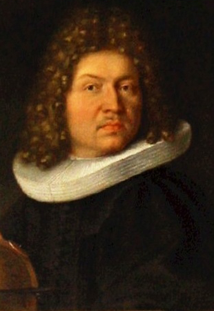
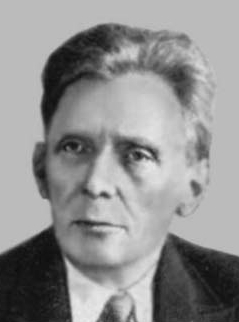
The law of large numbers and the central limit theorem have long and interesting histories. The weak law of large numbers for binomial (i.e. sums of Bernoulli) variables was first established by Jacob Bernoulli (1654–1705) and published in 1713 (Bernoulli 1713). The name ‘law of large numbers’ was given by Poisson. The modern version is due to Aleksandr Khinchin (1894–1959), and our Central Limit Theorem is only a special case—the assumption on variances is unnecessary.

It was apparent to mathematicians in the mid 1700s that a more refined result than Bernoulli’s law of large numbers could be obtained. A special case of the central limit theorem for binomial (i.e. sums of Bernoulli) variables was first established by de Moivre in 1733, and extended by Laplace; hence the normal approximation to the binomial is sometimes known as the de Moivre–Laplace theorem. The name ‘central limit theorem’ was given by George Pólya (1887–1985) in 1920.

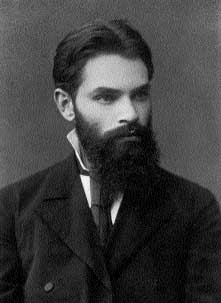
The first modern proof of the central limit theorem was given by Aleksandr Lyapunov (1857–1918) around 1901 (“Lyapunov Theorem,” n.d.). Lyapunov’s assumptions were relaxed by Jarl Waldemar Lindeberg (1876–1932) in 1922 (Lindeberg 1922). Many different versions of the central limit theorem were subsequently proved. The subject of Alan Turing’s (1912–1954) Cambridge University Fellowship Dissertation of 1934 was a version of the central limit theorem similar to Lindeberg’s; Turing was unaware of the latter’s work.