8 Expectation

🥅 Goals

Have an intuitive as well as mathematical understanding of expectation, variance, and covariance. Know how expectation, variance, and covariance, behave under linear transformations and sums.
Know how to evaluate expectation of functions of random variables.
Know the properties of expectation, variance, and covariance, and the relations between them.
Understand the difference between variance and standard deviation.
Know conditional expectation, the partition theorem for conditional expectation and the special notation associated with it.
Know how expectation, variance, and standard deviation behave under independence, and for sums of independent random variables in particular.
Know the Markov and Chebyshev inequalities, where they come from, and how to apply them.

8.1 Definition and interpretation

In a relative frequency interpretation (discussed earlier in Section 4.1), suppose that we run $n$ trials on an experiment where we observe the outcome of some real-valued random variable $X:\Omega\to\mathbb{R}$ in each trial. Let $x_i$ denote the observed value of $X$ in the $i$th trial; the sequence of observations $x_1$, $x_2$, …, $x_n$ is called a sample. The sample mean is then simply $\frac{1}{n}\sum_{i=1}^n x_i$. As a mathematical idealization, we may suppose that there is a unique, empirical limiting value for the sample mean, as $n$ tends to infinity, which we call the expectation of $X$.

In a betting interpretation (discussed earlier in ), you can simply consider your ‘fair price’ for a bet which pays $X$; that price, we call your expectation of $X$.

The idea of expectation is very interesting mathematically, and also provides ways to use probability in a host of practical applications. Regardless of interpretation, the expectation of $X$ can be connected to the probability mass function $p(x)$ (if $X$ is discrete) or the probability density function $f(x)$ (if $X$ is continuously distributed) in the following way:

🔑 Key idea: Definition: expectation

For any real-valued random variable $X$, the expectation (also called expected value or mean) of $X$, denoted as $\mathbb{E}[X]$, is defined as: \[\mathbb{E}[X]:= \sum_{x\in \mathcal{X}} x\; p(x) \tag{8.1}\] if $X$ is discrete, and \[ \mathbb{E}[X]:= \int_{-\infty}^\infty x\; f(x)\,dx \tag{8.2}\] if $X$ is continuously distributed, provided that the sum or integral exists.

Examples

Suppose that $X$ is discrete with probability mass function

$x$	$1$	$2$
$p(x)$	$\frac{1}{2}$	$\frac{1}{2}$

Then $\mathbb{E}[X] = \frac{1}{2} \cdot 1 + \frac{1}{2} \cdot 2 = 1.5$.

Consider the following ‘game’. You pay Jimmy a pound and then you both throw a fair die. If you get the higher number you get back the difference in pounds, otherwise you lose your pound. Call the return from a game $X$, with possible values 0, 1, 2, 3, 4 and 5. By counting outcomes,

$x$	$0$	$1$	$2$	$3$	$4$	$5$
$p(x)$	$\frac{21}{36}$	$\frac{5}{36}$	$\frac{4}{36}$	$\frac{3}{36}$	$\frac{2}{36}$	$\frac{1}{36}$

so that \[\mathbb{E}[X] = \sum_{x=0}^5 x\;p(x) = (0\times 21 + 1\times 5 + 2\times 4 + 3\times 3 + 4\times 2 + 5\times 1)/36 = 35/36.\] Since it costs £1 to play, this means that the expected profit is $-$£1/36. We can interpret this value as meaning that over a long series of games you will get back £35 for every £36 paid out.

To find the expectation of a discrete random variable $X$ where $p(x)=1/n$ for $x\in\{1,2,\dots,n\}$, we compute \[\begin{aligned} \mathbb{E}[X] &= \sum_{x=1}^n x p(x) \\ &= (1 + 2 + \cdots + n)\frac{1}{n} = \frac{n+1}{2} . \end{aligned}\]
If $X \sim \text{U}(a,b)$ then \[\mathbb{E}[X] = \int_a^b \frac{x}{b-a}\, dx = \left[\frac{x^2/2}{b-a}\right]_a^b = \frac{a+b}{2}. \]
If $Z \sim \mathcal{N}(0,1)$ then \[\mathbb{E}[Z]= \int_{-\infty}^{+\infty}z\phi(z) \, \mathrm{d} z = 0,\] since the integrand is an odd function ($\phi(z)=\phi(-z)$).

💪 Try it out

Find the expectation of a continuous random variable $X$ where \[f(x) = \begin{cases}x/2&\text{if }x\in[0,2], \\ 0&\text{elsewhere}.\end{cases}\]

Answer: We compute \[\mathbb{E}[X] = \int_0^2 x\cdot \frac{x}{2} \, \mathrm{d} x = \left[\frac{x^3}{6}\right]_0^2 = \frac{4}{3} . \]

Advanced content

If the range of possible values for a random variable $X$ is unbounded, then the sum or integral in may fail to exist. In this case, the preceding formulas may still be used to assign a meaningful expectation in some cases, provided we interpret them with care.

For example, if $X$ is discrete with probability mass function $p(x)$, consider \[\mathbb{E}[X]=\sum_{x\in X(\Omega) } x p(x) = \underbrace{\sum_{ x\in X(\Omega) : x \geq 0} x p(x)}_{S_+} + \underbrace{\sum_{ x\in X(\Omega) : x \leq 0} x p(x)}_{S_-} ;\] now the individual sums $S_+$ and $S_-$ always exist, but may be equal to $+\infty$.

In fact, if we write $X^+ = \max(X,0)$ and $X^- = \max(-X,0)$, then $X= X^+- X^-$ and $\mathbb{E}[X^+] = S_+$ and $\mathbb{E}[X^-] = S_-$.

To see this, note for example that $X^+$ is a random variable with $p_{X^+}{x} = p_X(x)$ for $x>0$ and $p_{X^+}(0) = \pr{ X \leq 0}$, but only the positive terms contribute to $\mathbb{E}[X^+]$.

It makes sense to say that $\mathbb{E}[X] = \mathbb{E}[X^+] - \mathbb{E}[X^-]$ (being possibly $-\infty$ or $+\infty$) as long as at most one of $S_+$ and $S_-$ are infinite, using the rules $\infty - x = \infty$ and $x - \infty = -\infty$ for finite $x$. (There is no sensible interpretation of $\infty - \infty$.) A similar argument applies in the continuous case, with integrals instead of sums. This is summarized in the following table, which shows the values of $\mathbb{E}[X]$ in each case.

	$\mathbb{E}[X^+] < \infty$	$\mathbb{E}[X^+] = \infty$
$\mathbb{E}[X^-] < \infty$	$\mathbb{E}[X^+] - \mathbb{E}[X^-]$	$+\infty$
$\mathbb{E}[X^-] = \infty$	$-\infty$	undefined

Examples

Suppose that $X$ is discrete with probability mass function $p(x) = c_\alpha x^{-\alpha}$ for $x \in \{1,2,\ldots\}$. This is only a proper probability mass function if $\zeta(\alpha):= \sum_{x=1}^\infty x^{-\alpha} < \infty$, so we need $\alpha > 1$. Then the normalizing constant must be $c_\alpha = 1/ \zeta(\alpha)$. But $\mathbb{E}[X] = c_\alpha \sum_{x=1}^\infty x^{1-\alpha}$. If $\alpha \in (1,2]$, this sum diverges, so $\mathbb{E}[X] = +\infty$. This is the case if, for instance, $p(x) = (6/\pi^2) x^{-2}$.

📖 Textbook references

If you want more help with this section, check out:

Sections 4.1 and 5.1 in (Blitzstein and Hwang 2019);
Section 3.3 in (Anderson, Seppäläinen, and Valkó 2018);
or Sections 4.3 and 7.4 in (Stirzaker 2003).

8.2 Expectation of functions of random variables

Let $X$ be a discrete random variable with $\pr {X \in \mathcal{X}}=1$ for a finite or countable set $\mathcal{X}$, and let $g: \mathcal{X}\to\mathbb{R}$ be a real-valued function. As seen in Section 6.11, $g(X):= g\circ X$ is again a random variable. Indeed, $g(X)$ is discrete, since $\pr{ g(X) \in g(\mathcal{X}) } =1$ where $g(\mathcal{X}) := \{ g(x) : x \in \mathcal{X} \}$ is finite or countable, and $g(X)$ is a real-valued random variable, so we can define its expectation.

To find the expectation of $g(X)$, by Equation 8.1, according to the definition we need to find the probability mass function $p_{g(X)}()$ first. It turns out however that we can express $\mathbb{E}[g(X)]$ directly in terms of $p_X()$, saving us the effort of having to calculate $p_{g(X)}()$ from $p_X()$.

For any $y\in g(\mathcal{X})$, \[\begin{aligned} p_{g(X)}(y) &=\pr{g(X)=y} =\sum_{x\in \mathcal{X}}\cpr{g(X)=y}{X=x}\pr{X=x} =\sum_{x \in \mathcal{X} : g(x)=y} p(x), \end{aligned} \tag{8.3}\] since \[\cpr{ g(X) = y}{X=x} = \begin{cases} 1 & \text{if } y = g(x), \\ 0 &\text{otherwise} .\end{cases}\] It follows that \[\begin{aligned} \mathbb{E}[g(X)] &=\sum_{y\in g(\mathcal{X})} y \, p_{g(X)}(y) =\sum_{y\in g(\mathcal{X})} y \left(\sum_{x \in \mathcal{X} : g(x)=y}p(x)\right) \\ & =\sum_{y\in g(\mathcal{X})} \left(\sum_{x \in \mathcal{X} : g(x)=y}yp(x)\right) =\sum_{x\in \mathcal{X}} \left(\sum_{y\in g(\mathcal{X}):y=g(x)} y p(x)\right) \\ & =\sum_{x\in \mathcal{X}} \left(\sum_{y\in g(\mathcal{X}):y=g(x)} y \right) p(x) =\sum_{x\in \mathcal{X}} g(x)p(x), \end{aligned}\] where we applied the definition of expectation, Equation 8.3, distributivity, change of order of summation, and distributivity again. A similar result can be proven when $X$ is continuously distributed. Concluding, we have the following result, which is sometimes known as the Law of the Unconscious Statistician:

Theorem: expectation of a function of a random variable

For any discrete random variable $X$ taking values in $\mathcal{X}$, and any function $g: \mathcal{X} \to\mathbb{R}$, \[\begin{aligned} \mathbb{E}[g(X)]&=\sum_{x\in \mathcal{X}} g(x)p(x) , \end{aligned} \tag{8.4}\] provided that the sum exists. Similarly, for any continuous random variable $X$ and any function $g: \mathbb{R} \to\mathbb{R}$, \[\begin{aligned} \mathbb{E}[g(X)]&=\int_{-\infty}^\infty g(x)f(x) \, \mathrm{d} x , \end{aligned} \tag{8.5}\] provided that the integral exists.

Examples

Suppose that $X$ takes values $0,1,2,3,4$ each with probability $1/5$. Then \[\begin{aligned} \mathbb{E}[(X-3)^2] &= \sum_{x=0}^4 (x-3)^2 p(x) \\ &= \frac{1}{5} ((0-3)^2 + (1-3)^2 + (2-3)^2 + (3-3)^2 + (4-3)^2) \\ &= \frac{1}{5}(9+4+1+0+1)=3. \end{aligned}\]
Suppose $X$ takes values $-2, -1, 0, 1, 2, 3$ each with probability 1/6. Then \[\begin{aligned} \mathbb{E}[X^2] &= \frac{1}{6}((-2)^2 + (-1)^2 + 0 + 1 + 2^2 + 3^2) = \frac{19}{6}; \\ \mathbb{E}[ \sin (\pi X/4) ] &= \frac{1}{6}(-1 - 1/\sqrt{2} + 0 + 1/\sqrt{2} + 1 + 1/\sqrt{2}) = \frac{1}{6\sqrt{2}}; \end{aligned}\] and so on.
If $X \sim \text{U}(-1, 1)$ then $f(x)=\frac{1}{2}$ for $x\in[-1,1]$, and zero elsewhere, so \[\begin{aligned} \mathbb{E}[X^2] & = \int_{-\infty}^\infty x^2 f(x) \, \mathrm{d} x \\ & = \int_{-1}^1 x^2\cdot\frac{1}{2} \, \mathrm{d} x \\ & = \left[ \frac{x^3}{6} \right]_{-1}^1 = \frac{1}{3} . \end{aligned}\]
Note that although $g(X)$ is discrete if $X$ is discrete, if $X$ is continuous then $g(X)$ need not be continuous: for example, if $X\sim\text{U}(0,2)$ and $g(x) = 1$ if $x \in (0,1)$ and $g(x) =0$ otherwise, we have that $g(X)$ is discrete with $\pr{ g(X) = 1} =1/2$ and $\pr{ g(X) = 0} =1/2$. In this case $f(x) = 1/2$ for $x \in (0,2)$, and says that \[\mathbb{E}[g(X)] = \frac{1}{2} \int_0^2 g(x) \, \mathrm{d} x = \frac{1}{2} ,\] as we would get from a direct calculation for the discrete random variable $g(X)$ as $\mathbb{E}[g(X)] = \frac{1}{2} \cdot 0 + \frac{1}{2} \cdot 1 = \frac{1}{2}$.

Advanced content

Similar comments apply here about extensions of $\mathbb{E}[g(X)]$ to include $+\infty$ or $-\infty$ as at the end of the previous section.

Example

Suppose $X \sim \text{U}(-1, 1)$ i.e., $X$ is uniformly distributed on the interval $(-1,1)$, and we set $g(x) =1/x$ for $x \neq 0$ and $g(0)=0$. Then $\mathbb{E}[g(X)]$ is not defined because $\mathbb{E}[g(X)^+] = \int_{-1}^0 0\,\frac{1}{2}\,dx + \int_0^1 \frac{1}{2x}\,dx = \infty$ and similarly $\mathbb{E}[g(X)^-] = \infty$.

For multiple random variables, the Law of the Unconscious Statistician reads as follows:

Expectation of a function of a multivariate random variable

For any discrete random variables $X$ and $Y$ taking values in $\mathcal{X}$ and $\mathcal{Y}$, and any function $g: \mathcal{X} \times \mathcal{Y} \to\mathbb{R}$, \[\begin{aligned} \mathbb{E}[g(X,Y)]&=\sum_{x\in \mathcal{X}} \sum_{y \in \mathcal{Y}} g(x,y)p(x,y) , \end{aligned}\] provided that the sum exists. Similarly, for any jointly continuously distributed random variables $X$ and $Y$, and any function $g: \mathbb{R}^2 \to\mathbb{R}$, \[\begin{aligned} \mathbb{E}[g(X,Y)]&=\iint\limits_{\mathbb{R}^2} g(x,y)f(x,y) \, \mathrm{d} x \, \mathrm{d} y, \end{aligned}\] provided that the integral exists.

Examples

Consider discrete random variables $X$ and $Y$ with joint probability mass function:

$p(x,y)$	$x=1$	$x=2$	$x=3$
$y=1$	$1/2$	$0$	$1/8$
$y=2$	$0$	$1/4$	$1/8$

Then \[\begin{aligned} \mathbb{E}[(X-2)Y] & = \sum_x \sum_y (x-2) y p(x,y) \\ & = (1-2) \cdot 1 \cdot \frac{1}{2} + (2-2) \cdot 2 \cdot \frac{1}{4} + (3-2) \cdot 1 \cdot \frac{1}{8} + (3-2) \cdot 2 \cdot \frac{1}{8} \\ & = -\frac{1}{8} . \end{aligned}\]

Consider discrete random variables $X$ and $Y$ with joint probability mass function:

$p(x,y)$	$x=-1$	$x=0$	$x=1$
$y=0$	$1/4$	$0$	$1/4$
$y=1$	$0$	$1/4$	$1/4$

Then $\mathbb{E}[XY] = \frac{1}{4}((-1)\times 0 + 0\times 1 + 1\times 0 + 1\times 1)= 1/4$.

💪 Try it out

Let $X$ and $Y$ be jointly continuously distributed random variables, with \[f(x,y) = \begin{cases} 1 & \text{if }(x,y)\in[0,1]^2, \\ 0 & \text{otherwise}. \end{cases}\] Find $\mathbb{E}[XY]$.

Answer:

Using the theorem, $\mathbb{E}[XY] = \int_0^1 \int_0^1 xy \, \mathrm{d} x \, \mathrm{d} y = (\int_0^1 x \, \mathrm{d} x) (\int_0^1 y \, \mathrm{d} y) = (1/2)^2 = 1/4$.

📖 Textbook references

If you want more help with this section, check out:

Sections 4.5 and 5.1 in (Blitzstein and Hwang 2019);
Section 3.3 in (Anderson, Seppäläinen, and Valkó 2018);
or Sections 4.5, 5.3, 7.4, and 8.5 in (Stirzaker 2003).

8.3 Linearity of expectation

Remember that summation and integration are linear operators, i.e., \[\begin{aligned} \sum_i \alpha f(x_i) + \beta g(x_i) &= \alpha \sum_i f(x_i) + \beta \sum_i g(x_i), \end{aligned}\] and \[\begin{aligned} \int_A \left( \alpha f(x)+\beta g(x) \right) \, \mathrm{d} x &= \alpha \int_A f(x) \, \mathrm{d} x + \beta \int_A g(x) \, \mathrm{d} x . \end{aligned}\] Consequently,

Theorem: linearity of expectation 1

For any real-valued random variable $X$, and any constants $\alpha$ and $\beta\in\mathbb{R}$, \[\mathbb{E}[\alpha X + \beta] = \alpha \mathbb{E}[X] + \beta .\]

A similar, but deeper, result is the following.

Theorem: linearity of expectation 2

For any two real-valued random variables $X$ and $Y$ on the same sample space $\Omega$, \[\mathbb{E}[X+Y] = \mathbb{E}[X]+\mathbb{E}[Y].\] More generally, for any real-valued random variables $X_1$, $X_2$, …, $X_n$, \[\mathbb{E}\left[\sum_{i=1}^n X_i \right] = \sum_{i=1}^n \mathbb{E}[X_i].\]

Proof

We give the proof in the case where $X$ and $Y$ are discrete. Consider the multiple random variable $(X,Y)$ and the function $g(x,y) = x+y$. By the Law of the Unconscious Statistician we get \[\begin{aligned} \mathbb{E}[g(X,Y) ] &= \sum_{x \in \mathcal{X}} \sum_{y \in \mathcal{Y}} (x+y) p(x,y) = \sum_{x \in \mathcal{X}} x \sum_{y \in \mathcal{Y}} p(x,y) + \sum_{y \in \mathcal{Y}} y \sum_{x \in \mathcal{X} } p(x,y) \\ & = \sum_{x \in \mathcal{X} } x p_X(x) + \sum_{y \in \mathcal{Y}} y p_Y(y) = \mathbb{E}[X] + \mathbb{E}[Y] , \end{aligned}\] as claimed. A similar calculation applies in the jointly continuous case, and the extension to more than two random variables follows by induction.

💪 Try it out

Suppose that $X\sim\text{Bin}(n,p)$. What is $\mathbb{E}[X]$?

Answer: We could use the probability mass function and compute \[\mathbb{E}[X] = \sum_{x=0}^n x p(x) = \sum_{x=0}^n \binom{n}{x} x p^x (1-p)^{n-x} ,\] but now some work is needed to evaluate this (exercise!).

Here is a neater way that will also be useful later on. Recall that $X$ counts the number of success on $n$ independent trails. If we let $Y_i = 1$ if trial $i$ is a success and $Y_i = 0$ if trial $i$ is a failure, then in the binomial scenario $Y_1, \ldots, Y_n$ are independent with $\pr{Y_i=1} =p$ and $\pr{Y_i=0}=1-p$. In other words, we may write \[X = Y_1 + Y_2 + \cdots + Y_n ,\] where $Y_i \sim\text{Bin}(1,p)$ are independent Bernoulli random variables. Then $\mathbb{E}[Y_i] = p$ and so $\mathbb{E}[X] = \mathbb{E}[Y_1 + \cdots + Y_n] = np$. Note that the independence of the trials is not necessary for this result.

Advanced content

We have proved linearity of expectation for discrete and jointly continuous random variables, but linearity of expectation is true for all random variables, and follows from the general measure-theoretic approach to probability theory, in which expectation is defined as a Lebesgue integral with respect to a probability measure; this includes the discrete and continuous settings we study as special cases. Students who take later probability courses will see some of this general approach. Note that without measure theory it is hard to prove the theorem in the case where say $X$ is discrete but $Y$ is continuous. If $X$ and $Y$ are independent, and at least one of them is continuous, then the sum $X+Y$ is also continuous: this is a theorem (see, e.g. (Moran 1968 Theorem 5.9, p.230)) and an example can be seen in Exercise 6.31, but this may fail without independence.

📖 Textbook references

If you want more help with this section, check out:

Section 4.2 in (Blitzstein and Hwang 2019);
Sections 4.2 and 4.6 in (DeGroot and Schervish 2013);
or Section 5.3 in (Stirzaker 2003).

8.4 Variance and covariance

As mentioned earlier, we can interpret the expectation of $X$ as a long-run average of a sample from distribution $X$. A popular and mathematically convenient way to measure the variability of $X$—i.e. to measure how much $X$ varies from $\mathbb{E}[X]$ in the long run—goes via the expectation of the random variable $(X-\mathbb{E}[X])^2$.

🔑 Key idea: Definition: Variance

Let $X$ be any real-valued random variable. The variance of $X$ is defined as \[\var{X}:= \mathbb{E}[\bigl( X-\mathbb{E}[X] \bigr)^2 ,\] and the standard deviation of $X$ is defined as \[\sd{X}:= \sqrt{\var{X}}.\]

Note that both $\var{X}$ and $\sd{X}$ are non-negative numbers.

Using LOTUS, we can immediately derive the following expressions for the variance: \[\begin{aligned} \var{X} &= \sum_{x\in \mathcal{X}} (x - \mathbb{E}[X])^2 p(x) &&\text{if $X$ is discrete, and} \\ \var{X} &= \int_{-\infty}^{\infty} (x - \mathbb{E}[X])^2 f(x) \, \mathrm{d} x &&\text{if $X$ is continuously distributed,} \end{aligned}\] provided that the sum or integral exists.

💪 Try it out

As in a previous example, suppose that $X$ takes values $0,1,2,3,4$ each with probability $1/5$. What is $\var{X}$?

Answer:

First we need to compute $\mathbb{E}[X]$, so \[\begin{aligned} \mathbb{E}[X] & =\sum_{x=0}^4x p(x)= \frac{0+1+2+3+4}{5} = \frac{10}{5} = 2. \end{aligned}\] Then \[\begin{aligned} \var{X} & = \sum_{x=0}^4(x-\mathbb{E}[X])^2p(x) \\ &= \frac{(-2)^2+(-1)^2+0^2+1^2+2^2}{5} = 2 . \end{aligned}\]

Examples

If $X$ takes values 0, 10, 20 each with probability 1/3, then \[\mathbb{E}[X]= 0\times \frac{1}{3} + 10\times \frac{1}{3} + 20\times\frac{1}{3} = 10.\] Consequently, using this value, \[\var{X} = \frac{1}{3}\times \left( (0-10)^2 + (10-10)^2 + (20-10)^2\right) = \frac{200}{3},\] and so $\sd{X} =\sqrt{\frac{200}{3}} \approx 8.16$.
Let $Z\sim\mathcal{N}(0,1)$. We know from an earlier example that $\mathbb{E}[Z]=0$ and by Exercise 8.x, $\mathbb{E}[Z^2]=1$. Consequently, \[\var{Z}=\mathbb{E}[(Z-E(Z)^2)]=\mathbb{E}[Z^2]=1,\] and $\sd{Z}=\sqrt{\var{Z}}=1$.

For two real-valued random variables, we can ask ourselves how they vary jointly.

🔑 Key idea: Definition:

Let $X$ and $Y$ be two real-valued random variables on the same sample space. The covariance of $X$ and $Y$ is defined as \[\cov{X,Y} := \mathbb{E}[ (X-\mathbb{E}[X])(Y-\mathbb{E}[Y]) ].\]

We also use the following qualitative terminology.

If $\cov{X,Y}>0$ it means that $X-\mathbb{E}[X]$ and $Y-\mathbb{E}[Y]$ tend to have the same sign. That is, if $X > \mathbb{E}[X]$ then it tends to be the case that $Y > \mathbb{E}[Y]$ (or, conversely, if $X < \mathbb{E}[X]$ then it tends to be the case that $Y < \mathbb{E}[Y]$ too). In this case we say that $X$ and $Y$ are positively correlated.
If $\cov{X,Y} <0$ we say that $X$ and $Y$ are negatively correlated. Now $X - \mathbb{E}[X]$ and $Y-\mathbb{E}[Y]$ tend to have opposite signs.
If $\cov{X,Y}=0$ we say that $X$ and $Y$ are uncorrelated.

Note: uncorrelated is not the same as independent (more on this later). A quantification of the correlation is provided by the correlation coefficient, given by \[\rho ( X, Y) := \frac{\cov{X,Y}}{\sqrt{ \var{X} \var{Y} } }.\] It can be proved (see Exercises 8.x and 8.x) that \[-1 \leq \rho(X,Y) \leq 1 .\] We will see an example below where the correlation coefficient is 1.

Using LOTUS for multiple random variables, we immediately derive the following expressions for the covariance: \[\cov{X,Y} = \sum_{x\in \mathcal{X}}\sum_{y\in \mathcal{Y}} (x - \mathbb{E}[X])(y - \mathbb{E}[Y]) p(x,y)\] if $X$ and $Y$ are discrete, and \[ \cov{X,Y} = \iint\limits_{\mathbb{R}^2} (x - \mathbb{E}[X])(y - \mathbb{E}[Y]) f(x,y) \, \mathrm{d} x \, \mathrm{d} y,\] if $X$ and $Y$ are jointly continuously distributed, provided that the double sum or double integral exists.

💪 Try it out

Consider discrete random variables $X$ and $Y$ with distribution given by

$p(x,y)$	$x=1$	$x=2$	$p_Y(y)$
$y=1$	$1/4$	$0$	$1/4$
$y=4$	$0$	$3/4$	$3/4$
$p_X(x)$	$1/4$	$3/4$

Find their expectations and their covariance.

Answer:

Then $\mathbb{E}[X] = 1 \cdot \frac{1}{4} + 2 \cdot \frac{3}{4} = \frac{7}{4}$ and $\mathbb{E}[Y] = 1 \cdot \frac{1}{4} + 4 \cdot \frac{3}{4} = \frac{13}{4}$. We compute, using the formula for expectation of a function (LOTUS again), \[\begin{aligned} \cov{X,Y} & = \mathbb{E}[\left( X - \frac{7}{4} \right) \left(Y - \frac{13}{4} \right) ] \\ & = \sum_x \sum_y \left( x - \frac{7}{4} \right) \left( y - \frac{13}{4} \right) p(x,y) \\ & = \frac{1}{4} \left( 1 - \frac{7}{4} \right) \left( 1 - \frac{13}{4} \right) + \frac{3}{4} \left( 2 - \frac{7}{4} \right) \left( 4 - \frac{13}{4} \right) \\ & = \frac{9}{16} . \end{aligned}\] This means that $X$ and $Y$ are positively correlated, which makes sense from the shape of the table.

We note two simple but important properties.

Proposition: Variance as covariance

For any real-valued random variable $X$, \[\var{X}=\cov{X,X}.\]

Proposition: Symmetry of covariance

For any real-valued random variables $X$ and $Y$, \[\cov{X,Y} =\cov{Y,X}.\]

As immediate consequences of linearity of expectation (see Section 8.3), we obtain the formulæ:

Corollary: Variance and covariance of linear combinations

For any real-valued random variable $X$, and any constants $\alpha$ and $\beta\in\mathbb{R}$,

\[ \var{\alpha+\beta X} = \beta^2\var{X}.\] For any real-valued random variables $X$, $Y$, and $Z$, and any constants $\alpha$, $\beta$, $\gamma$, and $\delta\in\mathbb{R}$, \[ \cov{\alpha + \beta X, \gamma + \delta Y} = \beta\delta\cov{X,Y}; \tag{8.6}\] \[ \cov{X+Y,Z} = \cov{X,Z} + \cov{Y,Z}; \tag{8.7}\] and \[\cov{X, Y+Z} = \cov{X,Y} + \cov{X,Z} \tag{8.8}\]

Note: Equation 8.6 through Equation 8.8 mean that $\cov{}$ is a bilinear operator.

Proof

We give an example of the type of calculation: \[\begin{aligned} \var{ \alpha + \beta X } & = \mathbb{E}[ \left(\alpha + \beta X - \mathbb{E}[\alpha + \beta X]\right)^2 ]\\ & = \mathbb{E}[ \left(\alpha + \beta X - \alpha - \beta \mathbb{E}[X]\right)^2 ]\\ & = \mathbb{E}[ \left( \beta X - \beta \mathbb{E}[X] \right)^2 ] \\ & = \beta^2 \mathbb{E}[(X - \mathbb{E}[X] )^2 ] \\ & = \beta^2 \var{X} . \end{aligned}\] The other statements are similar.

💪 Try it out

Let $X\sim\mathcal{N}(\mu,\sigma^2)$. Then, $Z:= \frac{X-\mu}{\sigma}\sim\mathcal{N}(0,1)$, and as we saw earlier, $\mathbb{E}[Z] = 0$ and $\var{Z}=1$. Consequently, \[\begin{aligned} \mathbb{E}[X]&=\expec{\mu+\sigma Z}=\mu + \sigma \mathbb{E}[Z] = \mu, \\ \var{X}&= \sigma^2 \var{Z} = \sigma^2. \end{aligned}\] In other words, the parameters $\mu$ and $\sigma^2$ of a normal distribution correspond to the expectation and variance, respectively.

We also obtain a slightly different way of calculating the variance:

Corollary: Variance and expectation

For any real-valued random variable $X$, \[\begin{aligned} \var{X} &= \expec{X^2} - \bigl(\mathbb{E}[X]\bigr)^2. \end{aligned}\]

Proof

Observe that, by linearity of expectation, \[\begin{aligned} \var{X} &= \expec{\left( X - \mathbb{E}[X] \right)^2 } \\ & = \expec{X^2 - 2X \mathbb{E}[X] +(\mathbb{E}[X])^2 } \\ &= \expec{X^2} - 2 \mathbb{E}[X] \mathbb{E}[X] + (\mathbb{E}[X])^2 \\ & = \expec{X^2} - (\mathbb{E}[X])^2, \end{aligned}\] as required.

Example

If $X$ takes values 0, 10, 20 each with probability 1/3, then \[\begin{aligned} \mathbb{E}[X] &= 0\times \frac{1}{3} + 10\times \frac{1}{3} + 20\times\frac{1}{3} = 10, \\ \expec{X^2} &= 0^2\times \frac{1}{3} + 10^2\times \frac{1}{3} + 20^2\times\frac{1}{3} = 500/3.\end{aligned}\] Consequently, \[\var{X} = \expec{X^2}-(\mathbb{E}[X])^2=100-500/3=200/3,\] which agrees with the value that we found earlier.

The next example shows how our various formulae can be put to good use.

💪 Try it out

Suppose that $X$ has probability mass function

$x$	0	3	10
$p(x)$	$1/4$	$1/2$	$1/4$

Define $Y = 2X-6$. Find

$\mathbb{E}[X]$, $\expec{X^2}$, and $\var{X}$;
$\mathbb{E}[Y]$ and $\var{Y}$;
$\cov{X,Y}$.

Answer:

For (a) we calculate that $\mathbb{E}[X] = 3 \cdot \frac{1}{2} + 10 \cdot \frac{1}{4} = 4$ and $\expec{X^2} = 3^2 \cdot \frac{1}{2} + 10^2 \cdot \frac{1}{4} = \frac{59}{2}$. So $\var{X} = \expec{X^2} - (\mathbb{E}[X])^2 = \frac{59}{2} - 4^2 = \frac{27}{2}$.

For (b), we compute swiftly that \[\mathbb{E}[Y] = \expec{2X - 6} = 2 \mathbb{E}[X] - 6 = 2 ,\] and \[\var{Y} = \var{2X-6} = 4 \var{X} = 54 .\]

Finally, for (c), \[\cov{X,Y} = \cov{ X, 2X-6} = 2 \cov{X,X} = 2 \var{X} = 27 .\] Note that \[\rho (X,Y) = \frac{\cov{X,Y}}{\sqrt{\var{X}\var{Y}}} = 1 ,\] which makes sense since $X$ and $Y$ are perfectly positively correlated.

We also obtain a slightly different way of calculating the covariance:

Corollary: Covariance via expectations

For any real-valued random variables $X$ and $Y$, \[\begin{aligned} \cov{X,Y} &= \mathbb{E}[XY] - \mathbb{E}[X]\mathbb{E}[Y]. \end{aligned}\]

Proof

The calculation should now be familiar: \[\begin{aligned} \cov{X,Y} & = \expec{(X-\mathbb{E}[X]) (Y-\mathbb{E}[Y] } \\ & = \expec{XY - Y \mathbb{E}[X] - X \mathbb{E}[Y] + \mathbb{E}[X] \mathbb{E}[Y] } \\ & = \expec{XY} - \mathbb{E}[Y]\mathbb{E}[X] - \mathbb{E}[X] \mathbb{E}[Y] + \mathbb{E}[X] \mathbb{E}[Y] \\ & = \mathbb{E}[XY] - \mathbb{E}[X] \mathbb{E}[Y], \end{aligned}\] as required.

Examples

We return to the previous example, with joint pmf given by

$p(x,y)$	$x=1$	$x=2$	$p_Y(y)$
$y=1$	$1/4$	$0$	$1/4$
$y=4$	$0$	$3/4$	$3/4$
$p_X(x)$	$1/4$	$3/4$

We already saw that $\mathbb{E}[X]=7/4$ and $\mathbb{E}[Y]=13/4$. Now we can compute $\mathbb{E}[XY] = \frac{1}{4} \cdot 1 + \frac{3}{4} \cdot 8 = \frac{25}{4}$, so that $\cov{X,Y} = \frac{25}{4} - \frac{7}{4} \cdot \frac{13}{4} = \frac{9}{16}$, as we obtained before.

Similarly to the preceding results, we have the following.

Corollary: Covariance of linear combinations

For any real-valued random variables $X$, $Y$, and $Z$
and any $\alpha$, $\beta$, $\gamma$, and $\delta\in\mathbb{R}$, \[\begin{aligned} \cov{\alpha + \beta X, \gamma + \delta Y} &= \beta\delta\cov{X,Y}, \\ \cov{X+Y,Z} &= \cov{X,Z} + \cov{Y,Z}, \\ \cov{X, Y+Z} &= \cov{X,Y} + \cov{X,Z}. \end{aligned}\]

💪 Try it out

Suppose $X$ takes values 0, 1, 2 with probabilities 1/4, 1/2, 1/4. Let $Y:= X^2$. What is $\var{X}$, $\var{Y}$, and $\cov{X,Y}$?

Answer:

First, $\mathbb{E}[X]=1$.

Next, $Y=X^2$ takes values 0, 1, 4 with probabilities 1/4, 1/2, 1/4, so $\expec{X^2}=\mathbb{E}[Y]=3/2$. Similarly, $Y^2=X^4$ takes values 0, 1, 16 with probabilities 1/4, 1/2, 1/4, so $\expec{Y^2}=9/2$. Finally, $XY=X^3$ takes values 0, 1, 8 with probabilities 1/4, 1/2, 1/4, so $\mathbb{E}[XY] = 5/2$. Concluding, \[\begin{aligned} \var{X} &= \expec{X^2}-(\mathbb{E}[X])^2=3/2-1=1/2; \\ \var{Y} &= \expec{Y^2}-(\mathbb{E}[Y])^2=9/2-9/4=9/4; \\ \cov{X,Y} &= \mathbb{E}[XY] - \mathbb{E}[X]\mathbb{E}[Y] = 5/2 - 3/2 = 1. \end{aligned}\]

Finally, we can now also say something about the variance of sums of random variables:

Theorem: Variance of a sum

For any real-valued random variables $X$ and $Y$ on the same sample space, \[\var{X+Y} = \var{X} + \var{Y} + 2\cov{X,Y}.\] More generally, for any real-valued random variables $X_1$, $X_2$, …, $X_n$, \[\var{\sum_{i=1}^n X_i} = \sum_{i=1}^n \var{X_i} + 2\sum_{i=1}^{n-1}\sum_{j=i+1}^n \cov{X_i,X_j}.\]

Proof

For the first statement, \[\begin{aligned} \var{X+Y} & = \cov{X+Y,X+Y} \\ & = \cov{X, X+Y} + \cov{Y,X+Y}\\ & = \cov{X,X} + \cov{X,Y} + \cov{Y,X} + \cov{Y,Y} , \end{aligned}\] which gives the result. In general, \[\begin{aligned} \var { \sum_{i=1}^n X_i } & = \cov { \sum_{i=1}^n X_i , \sum_{j=1}^n X_j }\\ & = \sum_{i=1}^n \cov { X_i , \sum_{j=1}^n X_j } \\ & = \sum_{i=1}^n \sum_{j=1}^n \cov { X_i, X_j } \\ & = \sum_{i=1}^n \cov{ X_i, X_i } + \sum_{i=1}^n \sum_{j \neq i} \cov {X_i, X_j} \\ & = \sum_{i=1}^n \var{X_i} + \sum_{i=1}^n \sum_{j=1}^{i-1} \cov{X_i, X_j} + \sum_{i=1}^n \sum_{j=i+1}^n \cov{X_i, X_j} , \end{aligned}\] with the convention that an empty sum is zero.

So, in general, the variance of a sum is not equal to the sum of the variances, unless all covariances are zero (zero covariance occurs under independence, covered later).

For example, for three real-valued random variables $X$, $Y$, and $Z$, \[\var{X+Y+Z} = \var{X} + \var{Y} + \var{Z} + 2\left( \cov{X,Y} + \cov{X,Z} + \cov{Y,Z} \right). \]

💪 Try it out

Suppose $X$ takes values 0, 1, 2 with probabilities 1/4, 1/2, 1/4. Let $Y:= X^2$.

We already found earlier that $\var{X}=1/2$, $\var{Y}=9/4$, and $\cov{X,Y}=1$. Now also find $\var{X+Y}$ and $\var{X-Y}$.

Answer:

By the above, $\var{X + Y} = \var{X} + \var{Y} + 2\cov{X,Y} = 1/2 + 9/4 + 2 \times 1 = 19/4$.

(Note that in this very simple example we can easily calculate $\var{X+Y}$ directly, as $X+Y$ takes possible values 0, 2, 6 with probabilities 1/4, 1/2, 1/4 so we can confirm by direct calculation that $\var{X+Y}=19/4$.)

Next, note that $\var{X - Y} = \var{X + Z},$ where $Z = -Y$. As $\var{Z} = (-1)^2\var{Y} = \var{Y}$ and $\cov{X,Z} = \cov{X,-Y} = -\cov{X,Y}$ we have \[\begin{aligned} \var{X - Y} &= \var{X} + \var{Y} - 2\cov{X,Y} \\ &= 1/2 + 9/4 - 2 \times 1 = 3/4. \end{aligned}\]

💪 Try it out

Suppose that $n$ people throw their hats high in the air, and each catches a hat which is equally likely to be any of the $n$ hats. Let $H$ be the number of men that catch their own hat. Find $\expec{H}$ and $\var{H}$.

Answer:

The distribution of $H$ is quite hard to find, but $\expec{H}$ and $\var{H}$ are fairly straightforward. Define \[X_i := \begin{cases} 1 & \text{if person $i$ catches their own hat}, \\ 0 & \text{otherwise}. \end{cases}\] Then $H=\sum_{i=1}^n X_i$. Here \[\expec{X_i} = \frac{1}{n} \times 1 + \frac{n-1}{n}\times 0 = \frac{1}{n},\] and so \[\expec{H} = \expec { \sum_{i=1}^n X_i } = \sum_{i=1}^n \expec{X_i} = 1 .\] Similarly, because $X_i^2=X_i$, \[\var{X_i} = \expec{X_i^2} - (\expec{X_i})^2 = \frac{1}{n} - \frac{1}{n^2} = \frac{n-1}{n^2} .\] We also need $\cov{X_i, X_j}$. We compute \[\begin{aligned} \expec{X_i X_j} &= \pr{X_i = 1, X_j = 1} \\ &= \pr{X_i = 1} \cpr{X_j = 1}{X_i = 1} \\ &= \frac{1}{n} \cdot \frac{1}{n-1} , \end{aligned}\] so \[\begin{aligned} \cov{X_i, X_j} &= \expec{X_i X_j} - \expec{X_i}\expec{X_j} \\ &= \frac{1}{n(n-1)} - \frac{1}{n^2} = \frac{1}{n^2(n-1)}. \end{aligned}\] Hence \[\begin{aligned} \var{H} &= \sum_{i=1}^n \var{X_i} + 2\sum_{i=1}^{n-1}\sum_{j=i+1}^n\cov{X_i, X_j} \\ &= n\var{X_1} + n(n-1) \cov{X_1, X_2} \\ &= n\times\frac{n-1}{n^2} + n(n-1)\times\frac{1}{n^2(n-1)} \\ &= \frac{n - 1 + 1}{n} = 1. \end{aligned}\]

📖 Textbook references

If you want more help with this section, check out:

Sections 4.6 and 7.3 in (Blitzstein and Hwang 2019);
Section 3.4 in (Anderson, Seppäläinen, and Valkó 2018);
or Sections 5.3, 5.3, and 8.5 in (Stirzaker 2003).

8.5 Conditional expectation

We now turn to the expectation of a random variable given an event (such as the value of another random variable). Recall that the indicator random variable of an event $A$ is given by \[𝟙\{A\}(\omega)= \begin{cases} 1&\text{if }\omega\in A, \\ 0&\text{otherwise}. \end{cases}\] Then $\expec{𝟙\{A\}}= 1 \cdot \pr{A} + 0 \cdot \pr{A^\textrm{c}} = \pr{A}$.

🔑 Key idea: Definition: conditional expectation

Let $X$ be a real-valued random variable, and let $A \subseteq \Omega$ be an event. The conditional expectation of $X$ given $A$ is: \[\cexpec{X}{A}:= \frac{\expec{X 𝟙\{A\}}}{\pr{A}}\text{ whenever }\pr{A}>0.\]

Conditional expectation generalizes the concept of conditional probability. For example, if $A$ and $B$ are any events such that $\pr{B}>0$ then because $𝟙\{A\}𝟙\{B\}=𝟙\{A\cap B\}$, it follows that $\expec{𝟙\{A\}\mid B}=\expec{𝟙\{A\}𝟙\{B\}}/\pr{B}=\pr{A\cap B}/\pr{B}=\cpr{A}{B}$.

One may also view $\cexpec{ \, \cdot \,}{A}$ as expectation with respect to the conditional probability $\cpr{ \, \cdot \,}{A}$:

🔑 Key idea: Theorem: conditional expectation and probabilities

For any discrete random variable $X$ and any event $A \subseteq \Omega$, \[\cexpec{X}{A} = \sum_{x \in \mathcal{X}} x \cpr{X=x}{A} .\]

Proof

This is an exercise in tracking definitions. Indeed, if $Y = X 𝟙\{A\}$, then for any $x \neq 0$, \[\pr{Y=x} = \pr{\{X=x\} \cap A} = \cpr{X=x}{A} \pr{A} .\] Hence \[\begin{aligned} \mathbb{E}[Y] & = \sum_{x \in \mathcal{X}} x \pr{Y=x} \\ & = \sum_{x \in \mathcal{X},\, x \neq 0} x \pr{Y=x} \\ & = \sum_{x \in \mathcal{X}} x \cpr{X=x}{A} \pr{A} , \end{aligned}\] and so \[\cexpec{X}{A} = \frac{\mathbb{E}[Y]}{\pr{A}} = \sum_{x \in \mathcal{X}} x \cpr{X=x}{A} ,\] as claimed.

💪 Try it out

Suppose that $X$ and $Y$ are discrete random variables, $g: \mathcal{X}\to\mathbb{R}$, and $B\subseteq \mathcal{Y}$. Then choosing the event $A = \{ Y \in B\}$, we see that whenever $\pr{Y\in B}=\sum_{y\in B}p_Y(y)>0$, \[\cexpec{g(X)}{Y\in B} = \frac{\sum_{x\in \mathcal{X}} g(x) \sum_{y\in B}p_{X,Y}(x,y)}{\sum_{y\in B}p_Y(y)} .\] As a special case, we have \[ \cexpec{g(X)}{Y=y}=\sum_{x\in \mathcal{X}} g(x)p_{X|Y}(x\vert y).\]

Similarly, if $X$ and $Y$ are jointly continuously distributed, then \[\cexpec{g(X)}{Y\in B} = \frac{\int_{\mathbb{R}}g(x) \left(\int_B f_{X,Y}(x,y)\, \mathrm{d} y\right)\, \mathrm{d} x}{\int_B f_Y(y)\, \mathrm{d} y},\] provided $\pr{Y\in B}=\int_B f_Y(y) \, \mathrm{d} y>0$.

To summarize, conditional expectation is just like ordinary expectation but with probabilities replaced by conditional probabilities.

💪 Try it out

In a raffle there is one £500 prize and five £100 prizes. We have one of the 2000 raffle tickets. Let $X$ be our winnings and let $A$ be the event that we have the top prize.

Calculate $\expec{X\mid A}$ and $\expec{X\mid A^\textrm{c}}$.
Compute $\cexpec{X}{A}\pr{A}+\cexpec{X}{A^\textrm{c}}\pr{A^\textrm{c}}$.
Compute $\mathbb{E}[X]$.

Answer:

By counting we see that $\cpr{ X = 500}{A} =1$ and \[\begin{aligned} \cpr{X = 500}{A^\textrm{c}} &=0, \\ \cpr{X = 100}{A^\textrm{c}} &= \frac{5}{1999}, \\ \cpr{X = 0}{A^\textrm{c}} & = \frac{1994}{1999} . \end{aligned}\] So we get $\cexpec{X}{A} = 500$ and \[\begin{aligned} \cexpec{X}{A^\textrm{c}} &= 100 \cdot \frac{5}{1999 } + 0 = \frac{500}{1999} . \end{aligned}\]

Now for(b), we note that $\pr{A}=1/2000$ and $\pr{A^\textrm{c}}=1999/2000$, so \[\cexpec{X}{A}\pr{A}+\cexpec{X}{A^\textrm{c}}\pr{A^\textrm{c}} = 500 \cdot \frac{1}{2000} + \frac{500}{1999} \cdot \frac{1999}{2000} = \frac{1000}{2000} = \frac{1}{2} .\] For (c), we compute directly that \[\mathbb{E}[X] = 500 \cdot \frac{1}{2000} + 100 \cdot \frac{5}{2000} + 0 = \frac{1}{2} .\] So the answers to (b) and (c) are the same.

It was no coincidence that the answers to parts (b) and (c) of were the same. This is an example of the following important theorem.

🔑 Key idea: Theorem: partition theorem for expectation

Let $X$ be any real-valued random variable. Let $E_1$, $E_2$, …, $E_k$ be any events that form a partition. Then, \[\mathbb{E}[X] = \sum_{i=1}^k \cexpec{X}{E_i} \pr{E_i}.\] Similarly, if $E_1$, $E_2$, …form an infinite partition \[\mathbb{E}[X] = \sum_{i=1}^\infty \cexpec{X}{E_i} \pr{E_i}.\]

Proof

Because $E_1, E_2, \ldots$ constitute a partition, $\cup_i E_i = \Omega$ and the $E_i$ are pairwise disjoint, so that \[1 = 𝟙\{\Omega\} = 𝟙\{\cup_{i} E_i\} = \sum_{i} 𝟙\{E_i\} ,\] and hence, by linearity of expectation, \[\mathbb{E}[X] = \expec{X\sum_{i} 𝟙\{E_i\} } = \sum_{i} \expec{X 𝟙\{E_i\} } ,\] which gives the result.

💪 Try it out

Ann and Bob play a sequence of independent games, each with outcomes $A = \{\text{Ann wins}\}$, $B =\{\text{Bob wins}\}$, $D = \{\text{game drawn} \}$ which have probabilities $\pr{A} = p$, $\pr{B} = q$ and $\pr{D} = r > 0$ with $p + q + r = 1$. Let $N$ denote the number of games played until the first win by either Ann or Bob. The results of the first game $A$, $B$, $D$ form a partition and $\cexpec{N}{A} = \cexpec{N}{B} = 1$ (as $\cpr{N = 1}{A}=\cpr{N=1}{B}= 1$) while $\cexpec{N}{D} = 1 + \expec{N}$ (the future after a drawn game looks the same as at the start). Hence $\expec{N} = 1\times p + 1\times q + (1 + \expec{N})\times r$ or $(1-r) \expec{N} = p + q + r = 1$ i.e. $\expec{N} = 1/(1-r)$.

A more demanding concept is the following:

🔑 Key idea: Definition: conditional expectation with respect to a random variable

Let $X$ be a real-valued random variable, and let $Y$ be another random variable. Define the function $g : Y(\Omega) \to \mathbb{R}$ by $g(y) := \cexpec{X}{Y=y}$. Then the conditional expectation of $X$ given $Y$ is the random variable denoted by $\cexpec{X}{Y}$ given by \[\cexpec{X}{Y} := g(Y).\]

You may see this written more compactly in books as \[\cexpec{X}{Y}(\omega) := \cexpec{X}{Y=Y(\omega)}, \text{ for all }\omega\in\Omega,\] but our definition above is a little easier to digest. In the case where $Y$ is discrete, $\cexpec{X}{Y}$ is a random variable that takes values $\cexpec{X}{Y=y}$ with probabilities $\pr{Y=y}$. We concentrate on the discrete case here.

The next result is of considerable importance.

🔑 Key idea: Theorem: partition theorem for expectation II

For any real-valued random variable $X$ and any random variable $Y$, \[\mathbb{E}[X]=\expec{\expec{X\mid Y}}.\]

Proof

We give a proof in the case when $Y$ is discrete, which shows why we call this a ‘Partition theorem’. In this case $\{ Y = y\}$, $y \in \mathcal{Y}$, forms a partition, and so gives \[\mathbb{E}[X] = \sum_{y \in \mathcal{Y}} \cexpec{X}{Y=y} \pr{Y=y } ,\] but this last expression is the expectation of the discrete random variable $\cexpec{X}{Y}$ which takes values $g(y) = \cexpec{X}{Y=y}$ with probabilities $\pr{Y=y }$: \[\expec{\expec{X\mid Y}} = \expec{g(Y) } = \sum_{y \in \mathcal{Y}} g(y) \pr {Y=y} ,\] by the law of the unconscious statistician.

This theorem is sometimes called the law of iterated expectation. We can use this result to calculate $\mathbb{E}[X]$ in some tricky cases.

💪 Try it out

Toss three fair coins and let $H$ be the total number of heads. The roll a fair die $H$ times, and let $T$ be the total score on the dice rolls. What is $\expec{T}$?

Answer:

This looks tricky, but we use conditioning on $H$ to take advantage of the structure of the problem. Note that $H\sim\text{Bin}(3, 1/2)$, so and $\expec{H}= 3/2$. Now, the expected score on a single die is \[\frac{1}{6} \left(1 +2 +3+4+5+6 \right) = \frac{7}{2} .\] Thus, given $h=h$, the expected total on $h$ rolls of a fair die the expected total score is $\frac{7}{2}h$. In other words, $\cexpec{T}{H=h} = \frac{7}{2}h$. Thus \[\cexpec{T}{H} = \frac{7}{2} H .\] Thus, by , \[\expec{T} = \expec{\expec{T \mid H}} = \frac{7}{2} \expec{H} = \frac{7}{2} \times \frac{3}{2} = \frac{21}{4} .\] Note that while this looks very slick, we have actually hidden something here. In fact, we have implicitly used the fact that the scores rolled on the die are independent of $H$, when we claimed that $\cexpec{T}{H=h} = \frac{7}{2}h$. To see where this is being used, let $S_1, S_2, \ldots$ be the scores on the die rolls, so $T = \sum_{i=1}^H S_i$. Then \[\cexpec{T}{H = h} = \cexpec{ \sum_{i=1}^{H} S_i}{H= h} =\cexpec{ \sum_{i=1}^h S_i }{ H = h } ,\] and we can drop the condition here if $H$ is independent of the $S_i$. Then \[\expec{T \mid H = h} = \expec{\sum_{i=1}^h S_i } =\sum_{i=1}^h \expec{S_i} = \frac{7}{2} h,\] as claimed. The next example is of the same type.

💪 Try it out

A shop has $N$ customers a day where $\expec{N} = 800$. Each customer spends £$X_i$ where $\expec{X_i} = 25$. Let $T = \sum_{i=1}^N X_i$ be the total takings on a particular day. What is $\expec{T}$?

Answer:

We condition on the value of $N$. Then \[\cexpec{T}{N = n} = \cexpec { \sum_{i=1}^n X_i }{N=n} .\] This is similar to the last example, and we must here use the fact that the $X_i$ are independent of $N$ to get \[\cexpec { \sum_{i=1}^n X_i }{N=n} = \expec{\sum_{i=1}^n X_i } = \sum_{i=1}^n \expec{X_i} = 25n .\] Thus $\cexpec{T}{N} = 25N$ and \[\expec{T} = \expec{\expec{T \mid N}} = \expec{25N} = 25\expec{N} = 25 \times 800 =20, 000 .\] In this example the assumption of independence between $N$ and the $X_i$ is open to question: if $N$ is very big, perhaps the $X_i$ might be smaller than usual, since the shop runs low on stock, for example.

📖 Textbook references

If you want more help with this section, check out:

Sections 9.1 and 9.2 in (Blitzstein and Hwang 2019);
Section 10.3 in (Anderson, Seppäläinen, and Valkó 2018);
or Sections 4.4 and 5.5 in (Stirzaker 2003).

8.6 Independence: multiplication rule for expectation

Remember that two discrete random variables are independent when their joint probability mass function factorises, i.e. when $p(x,y) = p(x) p(y)$. Similarly, two jointly continuously distributed random variables are independent when their joint probability density function factorizes, i.e. when $f(x,y) = f(x) f(y)$. It turns out that in these cases, expectation factorizes as well:

🔑 Key idea: Theorem: Independence means multiply

If $X$ and $Y$ are independent real-valued random variables then \[\mathbb{E}[XY]=\mathbb{E}[X]\mathbb{E}[Y].\] Moreover, if $g, h : \mathbb{R} \to \mathbb{R}$, \[\expec{g(X)h(Y)}=\mathbb{E}[g(X)]\expec{h(Y)}.\] More generally, for any mutually independent real-valued random variables $X_1$, $X_2$, …, $X_n$, \[\expec{\prod_{i=1}^n X_i} = \prod_{i=1}^n \expec{X_i}.\]

Proof

We give a proof only in the discrete case. Suppose that $X$ and $Y$ are independent discrete random variables with joint probability mass function $p(x,y) = p_X(x) p_Y(y)$. Then by the Law of the Unconscious Statistician, \[\expec{g(X)h(Y)} = \sum_{x \in \mathcal{X}} \sum_{y \in \mathcal{Y}} g(x) h(y) p(x,y) = \sum_{x \in \mathcal{X}} g(x) p_X(x) \sum_{y \in \mathcal{Y}} h(y) p_Y(y) ,\] which is $\mathbb{E}[g(X)] \expec{h(Y)}$.

Corollary: Independence means zero covariance

If $X$ and $Y$ are independent random variables, then $\cov{X,Y} = 0$.

Proof

In the independent case, $\cov{X,Y} = \mathbb{E}[XY] - \mathbb{E}[X]\mathbb{E}[Y] = 0$.

The converse of the last property is not true: $X$ and $Y$ may be dependent but uncorrelated.

Example

Suppose that $(X,Y)$ are jointly distributed taking values $(-1,0)$, $(+1,0)$, $(0,-1)$, and $(0,+1)$ with probability $1/4$ of each. Then $X$ and $Y$ are not independent, because $\pr{X=1, Y=1} = 0$ is not the same as $\pr{X=1} \pr{Y=1} = 1/16$, for instance. However, $X$ and $Y$ are uncorrelated, because $\mathbb{E}[XY] = 0$ and $\mathbb{E}[X]=\mathbb{E}[Y]=0$ so $\cov{X,Y}=0$. (In fact, in this case $XY=0$ with probability 1.)

An important consequence of this Corollary is a simplification of the formula for the variance of a sum for pairwise independent random variables:

Corollary: Variance of a sum of independent variables

Consider random variables $X_1$, $X_2$, …, $X_n$. If these random variables are pairwise independent, then \[\var{\sum_{i=1}^n X_i} = \sum_{i=1}^n \var{X_i}.\]

Example

Remember from an earlier example that we can write any $X\sim\text{Bin}(n, p)$ as $X=\sum_1^n Y_i$ where $Y_1$, …, $Y_n$ are independent and each $Y_i\sim\text{Bin}(1,p)$. In , you showed that $\var{Y_i} = p(1-p)$. Consequently, as the $Y_i$ are independent, \[\var{X}=\sum_{i=1}^n\var{Y_i}=np(1-p). \]

💪 Try it out

Let $S$ be the total score and $T$ be the product of the scores from throwing four dice.

To find $\expec{S}$, $\var{S}$ and $\expec{T}$ let the individual scores be $X_k$, $k = 1$, 2, 3, 4 so that $S = \sum_{k=1}^4 X_k$, $T = \prod_{k=1}^4 X_k$.

We readily calculate $\expec{X_k} = \sum_{i=1}^6 i \times 1/6 = 7/2$ and $\var{X_k} = \sum_{i=1}^6 i^2 \times 1/6 - (7/2)^2 = 35/12$. Therefore \[\expec{S}= \expec { \sum_{k=1}^4 X_k } = \sum_{k=1}^4 \expec{X_k} = 4\times 7/2 = 14,\] and further, as the $X_k$ are independent, \[\var{S} = \var{\sum_{k=1}^4 X_k} = \sum_{k=1}^4 \var{X_k} = 4 \times 35/12 = 35/3.\] Again as the $X_k$ are independent, \[\expec{T} = \expec { \prod_{k=1}^4 X_k } = \prod_{k=1}^4 \expec{X_k} = \left( \frac{7}{2} \right)^4 = 2401/16.\] Note that all of these calculations are possible without having to deal with the joint probability distribution of the $X_k$ (which is uniform on the 1296 possible outcomes).

📖 Textbook references

If you want more help with this section, check out:

Section7.3 in (Blitzstein and Hwang 2019);
Section 8.2 in (Anderson, Seppäläinen, and Valkó 2018);
or Section 5.3 in (Stirzaker 2003).

8.7 Expectation and probability inequalities

By the monotonicity properties of summation and integration, namely that if $f(x) \geq g(x)$ then \[\begin{aligned} \sum_i f(x_i) \geq \sum_i g(x_i), \text{ and } \int_A f(x) \, \mathrm{d} x \geq \int_A g(x) \, \mathrm{d} x , \end{aligned}\] we immediately get the following.

Theorem: Monotonicity of expectation

For any random variable $X$, and any $a\in\mathbb{R}$, if $\pr { X\geq a } =1$ then $\mathbb{E}[X]\geq a$.

For instance, suppose that $X$ and $Y$ have $\pr { X \leq Y } = 1$. Then $\pr{ Y-X \geq 0 } =1$ so $\expec{Y - X} \geq 0$ and hence $\mathbb{E}[X] \leq \mathbb{E}[Y]$.

This simple property has various interesting consequences:

Corollary: Variances are positive

For any random variable $X$, $\var{X} \geq 0$.

Proof

We have $\var{X} = \expec{(X-\mathbb{E}[X])^2 }$ and the random variable $(X-\mathbb{E}[X])^2$ is non-negative.

🔑 Key idea: Corollary: Markov's inequality

If $X\geq 0$ then, for any $a>0$, \[\pr{X \geq a} \leq \frac{\mathbb{E}[X]}{a}.\]

Proof

Note that $X\geq a 𝟙\{X\geq a\}$, and consequently $0\le \expec{X-a 𝟙\{X\geq a\}}=\mathbb{E}[X]-a\pr{X\geq a}$.

Example

If $X$ equals $s$ with chance $p$ but otherwise equals 0 then $\mathbb{E}[X] = sp$. For $a > s$ we have $0 = \pr{X \geq a} \leq ps/a$ while for $a \leq s$ Markov’s inequality says $p = \pr{X \geq a} \leq p\times s/a$ which is exact at $a = s$ so this bound is as strong as possible.

Corollary: Chebyshev's inequality

For any random variable $X$ and any $a>0$, we have \[\pr { |X-\mathbb{E}[X]| \geq a } \leq \frac{\var{X}}{a^2}.\]

Proof

$\pr { (X-\mathbb{E}[X])^2 \geq a^2 } \leq \expec{(X - \mathbb{E}[X])^2 }/a^2$ by Markov’s inequality applied to $(X-\mathbb{E}[X])^2$ at $a^2$. Now observe that $\{ (X-\mathbb{E}[X])^2 \geq a^2 \} = \{ |X-\mathbb{E}[X]| \geq a \}$ and of course $\mathbb{E}[(X - \mathbb{E}[X])^2 ] = \var{X}$.

Markov and Chebyshev bounds are often too generous when distributional information is available, as seen in the next examples. Nevertheless, their generality and simplicity make these inequalities very valuable for complex probability calculations.

💪 Try it out

Suppose that $X\sim\text{Bin}(10,0.1)$. Give an upper bound on $\pr{X \geq 6}$ using (a) Markov’s inequality, and (b) Chebyshev’s inequality.

Answer:

For part (a), we get \[\pr{X \geq 6} \leq \frac{\mathbb{E}[X]}{6} = \frac{1}{6} .\] For (b), we get \[\begin{aligned} \pr {X \geq 6} & \leq \pr { | X-1| \geq 5 } \\ & = \pr { | X-\mathbb{E}[X] | \geq 5} \\ & \leq \frac{\var{X}}{25} = \frac{0.9}{25} =0.036 . \end{aligned}\] The exact probability can be calculated and is $\pr { X \geq 6} \approx 0.00015$.

💪 Try it out

If $Z \sim \mathcal{N}(0, 1)$ then $\pr { |Z - \mathbb{E}[Z]| \geq 2} = \pr{|Z| \geq 2} = 1 - \pr{-2 < Z < 2} = 0.046$, while the Chebyshev bound on this probability is $\var{Z}/2^2 = 0.25$.

📖 Textbook references

If you want more help with this section, check out:

Section 10.1 in (Blitzstein and Hwang 2019);
Section 4. in (DeGroot and Schervish 2013);
or Section 4.6 in (Stirzaker 2003).

8.8 Historical context

There are approaches to probability theory that start out from expectation of random variables directly, rather than starting out from probability of events as we have done here; see e.g. (Whittle 1992).

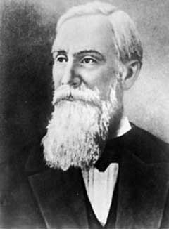
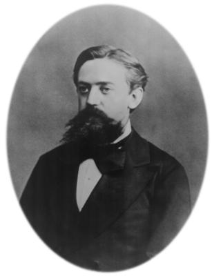
Pafnuty Chebyshev (1821–1894) and his student Andrei Markov (1856–1922) made several important contributions to early probability theory. What we call Markov’s inequality was actually published by Chebyshev, as was what we call Chebyshev’s inequality; our nomenclature is standard, and at least has the benefit of distinguishing the two. A version of the inequality was first formulated by Irénée-Jules Bienaymé (1796–1878).

	\(\mathbb{E}[X^+] < \infty\)	\(\mathbb{E}[X^+] = \infty\)
\(\mathbb{E}[X^-] < \infty\)	\(\mathbb{E}[X^+] - \mathbb{E}[X^-]\)	\(+\infty\)
\(\mathbb{E}[X^-] = \infty\)	\(-\infty\)	undefined

\(p(x,y)\)	\(x=1\)	\(x=2\)	\(x=3\)
\(y=1\)	\(1/2\)	\(0\)	\(1/8\)
\(y=2\)	\(0\)	\(1/4\)	\(1/8\)

\(p(x,y)\)	\(x=-1\)	\(x=0\)	\(x=1\)
\(y=0\)	\(1/4\)	\(0\)	\(1/4\)
\(y=1\)	\(0\)	\(1/4\)	\(1/4\)

\(p(x,y)\)	\(x=1\)	\(x=2\)	\(p_Y(y)\)
\(y=1\)	\(1/4\)	\(0\)	\(1/4\)
\(y=4\)	\(0\)	\(3/4\)	\(3/4\)
\(p_X(x)\)	\(1/4\)	\(3/4\)

\(p(x,y)\)	\(x=1\)	\(x=2\)	\(p_Y(y)\)
\(y=1\)	\(1/4\)	\(0\)	\(1/4\)
\(y=4\)	\(0\)	\(3/4\)	\(3/4\)
\(p_X(x)\)	\(1/4\)	\(3/4\)